
Investment Appraisal Under Uncertainty

1 Introduction
Long-term decisions such as capital investment appraisal are taken on estimates. Whatever the appraisal method — payback, ARR, IRR or NPV — the figures are projections of the future and cannot be known with certainty.
There is always a risk that the estimates will not match what actually happens. If some of the projected cash flows turn out to be different from the ones used in the decision, the decision itself may no longer be the right one.
This chapter deals with the techniques that measure that exposure and build it into the appraisal: sensitivity analysis, simulation, stress testing, expected values, the standard deviation of the return, value at risk, and the risk-adjusted discount rate.
Chapter 16 applies several of the same techniques — expected values, sensitivity analysis and the decision rules — to business decisions generally rather than to capital projects, and adds decision trees and the value of perfect information.
2 Sensitivity analysis
Sensitivity analysis appraises an investment whose outcome depends on a number of uncertain input variables. A decision to invest in a new machine, for example, rests on estimates of sales demand, the selling price, the contribution per unit, the labour hours, the fixed costs and the cost of capital.
Sensitivity measures the responsiveness of the decision to a change in each variable taken one at a time. It tells you how crucial each estimate is to the accept/reject decision, and therefore which estimates deserve the most work before the project is approved.
This lecture works Example 1 in full and then introduces simulation (section 3). It teaches the 2027 outcome as written. It stops there: the stress testing in section 4 is not on tape, and no P2 recording covers it.
2.1 The method
Calculate the NPV of the project on the estimated figures.
Identify every input variable the NPV depends on.
For each variable in turn, holding everything else constant, calculate the percentage change in that variable that would bring the NPV down to zero.
Zero is the break-even point of the decision: any change larger than that percentage turns a positive NPV negative and so turns the decision from accept to reject. The percentage is therefore the margin of error the estimate can carry.
Key point
Sensitivity of a variable = NPV ÷ present value of the flow that variable affects, as a percentage.
Sensitivity = (NPV ÷ PV of the flow affected) × 100%
The rule works because a change in one variable changes the present value of the flow it drives in the same proportion. If sales volume falls by 5%, total contribution falls by 5%, and so does its present value. So the question "what percentage change wipes out the NPV?" becomes "the NPV is what percentage of the present value that would move?".
The cost of capital is the exception. A change in the discount rate changes every discounted flow at once, so there is no single "flow affected". Instead, find the discount rate at which the NPV is zero — that is the IRR by definition — and express the gap between the IRR and the estimated cost of capital as a percentage of that estimate.
Give every answer a direction. A sensitivity is a one-way margin. For a cost or an outflow the danger is that it turns out higher, so the answer is positive; for revenue, volume, contribution or a scrap receipt the danger is that it turns out lower, so the answer is negative. Movement the other way makes the project better, not worse.
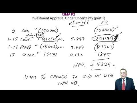
Daina has just set up a new company and estimates that the cost of capital is 15%.
Her first project involves investing $150,000 in equipment with a life of 15 years and a final scrap value of $15,000.
The equipment will produce 15,000 units a year, generating a contribution of $2.75 each. She estimates that additional fixed costs will be $15,000 a year.
(a) Determine, on the basis of the above figures, whether the project is worthwhile.
(b) Calculate the sensitivity to change of:
(i) the initial investment
(ii) the sales volume per annum
(iii) the contribution per unit
(iv) the fixed costs per annum
(v) the scrap value
(vi) the cost of capital
(c) Comment on the results.
Show answerHide answer
2.2 Advantages and limitations of sensitivity analysis
Advantages | Limitations |
It identifies the critical variables, so scarce forecasting effort is spent where the decision is actually at risk. | Each variable is flexed on its own. In practice several move at the same time, and a much smaller change in two of them together can reverse the decision. |
It needs no probability estimates and is calculated from an NPV that has already been prepared. | It says nothing about how likely a change is. A 2% sensitivity on a stable variable may matter less than a 20% sensitivity on a volatile one, and sensitivity analysis cannot tell them apart. |
It expresses risk in terms a non-financial manager can act on: how wrong can this estimate be before the answer changes? | The variables are often related — selling price and volume, volume and variable cost — so holding one constant while flexing another is artificial. |
It supports a decision to reject a project that has a positive NPV but no margin of safety, which an NPV on its own never does. | It does not make the decision. What counts as too small a margin still depends on the decision-maker's attitude to risk. |
3 Simulation and the Monte Carlo method
Simulation answers the main criticism of sensitivity analysis: it looks at the effect of changes in more than one variable at the same time.
Applied to investment appraisal, Monte Carlo simulation software produces a distribution of NPV outcomes for a project with many input variables, each with its own uncertainty, rather than a single figure.
3.1 The stages
Identify the major variables.
Specify the relationships between them.
Attach a probability distribution to each variable, and assign random numbers to reflect it.
Simulate one outcome by generating a random combination of values and computing the NPV.
Record the result.
Repeat the simulation many thousands of times to build a probability distribution of the possible NPVs.
The output is not a single NPV but a distribution: the mean NPV, the spread around it, and — the figure a board usually asks for — the probability that the NPV is negative.
Exam expectation. You will not be asked to perform a simulation. You are expected to know what it does, what it needs (a distribution for every variable, and the relationships between them) and why its output is more informative than a sensitivity table.
4 Stress testing a project
Sensitivity analysis asks how far one estimate can move. A stress test asks a different question: what happens to this project if a plausible set of bad things happens at once?
A stress test therefore flexes several variables together, to a severe but credible level, and reports what the project looks like in that state. Typical forms are:
Scenario analysis — a small number of internally consistent scenarios (say optimistic, most likely and pessimistic), each with every variable set to a value that is consistent with the others. Unlike sensitivity analysis, the variables are allowed to move together, which is what actually happens.
A worst-case combination — every critical variable set to the far end of its plausible range at the same time, to see whether the entity could survive the outcome rather than whether the project would still be accepted.
A specific shock — the loss of the largest customer, a doubling of an input price, a two-year delay in commissioning, a cyber incident that halts production for a month.
Reverse stress testing — start from the failure and work back: what combination of outcomes would make this project unaffordable, and how likely is that combination?
The point of a stress test is not to produce a better NPV. It is to establish whether a bad outcome would be survivable, what the entity would do about it, and whether that response should be arranged now — a break clause, a phased commitment, a hedge, a contingency reserve.
Chapter 17 applies the same idea at the level of the whole business rather than the single project.
5 Expected values
Where a variable can take a small number of values and the probability of each is known, the uncertain figure can be replaced by its probability-weighted average — its expected value — and the appraisal then proceeds normally.
EV = Σpx
where x is each possible outcome and p is its probability.
This lecture works Example 2. One correction: at the point where the tutor totals the expected fixed overheads he says “258,000”; the figure is $158,000, which is what he then uses in the discounting and what the answer below shows. He also leaves part (b) to be checked against the printed answer rather than discounting it on screen.

Daiga plc is considering launching a new product. This will require additional capital investment of $200,000.
The selling price of the product will be $10 per unit. Daiga has ascertained that the probability of a demand of 50,000 units a year is 0.5, with a probability of 0.4 that it will be 20% higher and a probability of 0.1 that it will be 20% lower.
The company expects to earn a contribution of 50% of selling price and expects fixed overheads to increase by $140,000 a year.
The time horizon for appraisal is 4 years. The machine will be sold at the end of 4 years for $50,000. The cost of capital is 20% a year.
(a) Calculate the expected NPV of the project.
(b) Assuming that demand is certain at 50,000 units a year, calculate the expected NPV of the project if fixed overheads are uncertain as follows:
Fixed overheads $ | Probability |
100,000 | 0.20 |
140,000 | 0.35 |
180,000 | 0.25 |
220,000 | 0.20 |
Show answerHide answer
5.1 The limitation of an expected NPV
An expected value is a long-run average. Daiga will not receive an NPV of $147,725, because demand will not be 53,000 units — it will be 50,000, 60,000 or 40,000. The expected NPV is the average the project would produce if it were repeated many times under the same conditions, and a capital project is normally a one-off.
It is still the best single figure available, but it hides the spread of the outcomes entirely — which is what the standard deviation is for.
6 Standard deviation and the coefficient of variation
Two projects can have the same expected NPV and be quite different propositions. If project A and project B both have an expected NPV of $40,000 but A's standard deviation is $2,000 and B's is $6,500, A's outcome is likely to land much closer to $40,000 than B's.
Standard deviation measures dispersion — how far, on average, the possible outcomes lie from the expected value. The higher the standard deviation, the wider the spread of outcomes and so the higher the risk.
This lecture works Example 3 and explains the formula term by term. It teaches the 2027 outcome correctly.

6.1 The formula
σ = √[Σ p(x − x̄)2]
where x is each possible outcome, p is its probability and x̄ is the expected value, Σpx.
Work it in columns. The squaring removes the sign, so that positive and negative deviations do not cancel to nil; the square root at the end returns the answer to the units of the original data — percentages if the outcomes were percentages, dollars if they were dollars.
x | p | px | x – x̄ | p(x – x̄)² |
each outcome | its probability | multiply | deviation from the mean | square the deviation, multiply by p |
Add the px column to get the expected value; add the last column to get the variance; take the square root of the variance to get the standard deviation.
6.2 The coefficient of variation
A standard deviation on its own does not say whether the spread is large. A spread of 3.5% is trivial against returns of 80% to 100% and enormous against returns of 1% to 3%. The coefficient of variation scales it against the mean, so that two investments of different sizes can be compared.
Coefficient of variation = σ ÷ x̄
The following are the likely returns from project Z.
Return | Probability |
10% | 0.2 |
15% | 0.5 |
20% | 0.3 |
Calculate the expected value and the standard deviation for project Z.
What is the coefficient of variation in this case?
Show answerHide answer
7 Value at risk (VaR)
Beyond the core
Value at risk is not one of the techniques the 2027 P2 syllabus names. P2D1's topics are the quantification of risk, probabilistic models, stress-testing, decision trees and decision-making under uncertainty; VaR is normally met as a financial-risk technique in F3. It is kept here as background, because it is the natural extension of the standard deviation you have just calculated, and because it is how a bank or a treasury function states risk in one number.
An investor is usually less interested in the spread of outcomes in general than in one specific question: how much could I lose? Value at risk answers it.
Value at risk is the loss that will not be exceeded, over a stated holding period, at a stated confidence level. The holding period is usually short — one to ten days. Confidence levels are usually 95% to 99%: at 95%, VaR is the amount that has a 5% chance of being exceeded during the period.
7.1 Calculating it
Where the outcomes are normally distributed, VaR is a multiple of the standard deviation. The multiple is the number of standard deviations that leaves the chosen tail probability beyond it.
VaR = z × σ
Confidence level | Tail probability | z (one-tailed) |
95% | 5% | 1.645 |
97.5% | 2.5% | 1.960 |
99% | 1% | 2.326 |
The standard deviation must be measured over the same period as the holding period. Where it is quoted for a different period and returns are assumed independent, it is scaled by the square root of time — a daily standard deviation is multiplied by √10 for a ten-day holding period.
A bank has estimated that the expected value of its portfolio in 2 weeks' time will be $100 million, with a standard deviation of $5 million.
Estimate the value at risk at a 95% confidence level.
Show answerHide answer
7.2 What VaR does not tell you
It is silent about the size of the loss in the tail beyond the confidence level, which is the loss that actually causes failures.
It assumes the distribution — normally the normal distribution — and real returns have fatter tails than that, so extreme losses are more frequent than the model implies.
It is calibrated on past volatility, and volatility is not stable: the periods when VaR matters most are exactly the periods in which yesterday's standard deviation understates today's risk.
8 Risk-adjusted discount rates
The risk in a project depends on its context: the strength of the competition, the type of investment, the volatility of the market. Some projects are plainly riskier than others — the acquisition of a foreign business is likely to be riskier than an expansion of existing domestic operations.
Higher risk does not make a project worse. The foreign acquisition may deliver a much higher return; it may equally deliver a low or negative one. What higher risk does is raise the return the investor requires.
One response is therefore to discount a higher-risk project at a higher cost of capital, adding a risk premium to the entity's normal discount rate. Rational investors accept higher risk only where the expected return is higher, and a risk-adjusted rate builds that requirement into the appraisal: a risky project must clear a higher hurdle before its NPV turns positive.
The weakness of the method is the premium itself. Unless it is derived from something observable — the returns required on quoted entities in the same line of business, for example — it is chosen by judgement, and a discount rate chosen by judgement can be made to produce whatever answer is wanted. It also penalises later cash flows more heavily than earlier ones, which is only correct if the risk really does compound with time.
Where the risk is confined to one variable, adjusting that cash flow — by an expected value, or by the stress test in section 4 — is more transparent than adjusting the rate that discounts all of them.
9 Chapter summary
Technique | Question it answers | What it needs |
Sensitivity analysis | How far can one estimate be wrong before the decision changes? | An NPV |
Simulation (Monte Carlo) | What is the distribution of NPVs when every variable moves at once? | A probability distribution for each variable, and software |
Stress testing | Could the entity survive a severe but plausible combination of bad outcomes? | Internally consistent scenarios |
Expected values | What is the single best estimate of an uncertain variable? | Outcomes and their probabilities |
Standard deviation / coefficient of variation | How wide is the spread of outcomes, absolutely and relative to the mean? | Outcomes and their probabilities |
Value at risk (beyond the core) | How much could be lost over a short holding period, at a stated confidence level? | A standard deviation and a distribution assumption |
Risk-adjusted discount rate | What return should this project have to earn to compensate for its risk? | A defensible risk premium |
10 Test your knowledge
Two quick checks before you move on: work through the flashcards to fix this chapter’s key terms and definitions, then sit the objective questions for exam-style practice. Both mark themselves and explain the answers as you go.
Investment Appraisal Under Uncertainty
11 questionsAnswer the questions one at a time. Your progress is saved so you can leave and come back.
Open chapter practice