
Risk and Uncertainty

1 Introduction
Business decisions are choices made now about outcomes that will happen later, and later outcomes are rarely known with certainty. New product launches, capital investments, contract negotiations and capacity decisions are all taken without any guarantee of the result.
Risk exists whenever the actual outcome of a decision may differ from the forecast one. This chapter deals with the techniques used to make a decision anyway, and to say afterwards why that decision was the right one on the information available.
Chapter 15 applied expected values, sensitivity analysis and the standard deviation to capital investment appraisal specifically. Here the same techniques are applied to business decisions generally, and two more are added: the decision rules for choosing between courses of action, and decision trees.
2 Risk and uncertainty
The two words are often used interchangeably, but there is a technical difference and it matters because it decides which techniques are available.
Risk | Uncertainty |
Can be quantified. The possible outcomes are known and a probability can be attached to each. A roll of a die is the standard illustration: the result is unknown, but there are exactly six outcomes and each has a probability of 1/6. | Cannot be quantified. There is no well-defined set of possible outcomes, and no reliable probabilities. Whether a technology now being developed will exist in ten years, and what it will do to this market, is uncertainty. |
Expected values, standard deviation, decision trees and simulation all need probabilities, so they belong to risk. | Maximax, maximin and minimax regret need no probabilities at all, so they are what is left when the situation is genuinely uncertain. |
Most real decisions sit between the two: the outcomes can be listed, but the probabilities attached to them are themselves estimates. That is worth remembering whenever an expected value is calculated to the nearest dollar.
3 Attitudes to risk
Faced with the same numbers, two managers can reasonably make different decisions, because the choice depends on attitude to risk as well as on arithmetic. There is no best attitude and no best decision rule; in the examination you apply whichever rule you are told to apply.
Attitude | What the decision-maker looks at | Decision rule that expresses it |
Risk seeker | The best possible outcome, however small the chance of achieving it. Optimistic — and reckless if the likelihood of the outcome is ignored altogether. | Maximax |
Risk neutral | The most likely, or average, outcome. Balances risk against reward. | Expected value |
Risk averse | The worst possible outcome. Of two choices, takes the less risky one even where the expected return is lower. | Maximin |
Minimax regret belongs to none of the three. It is the rule of the decision-maker who is not worried about the outcome itself but about the opportunity lost — about looking back and finding that another choice would have been better.
4 Expected values
An expected value can be calculated wherever a decision has several possible outcomes and the probability of each is known. It is the probability-weighted average of the outcomes.
EV = Σpx
The expected value represents a long-run average: the result the decision-maker would get, on average, if the same decision were taken many times over.
This recording covers sections 2 to 5 — risk and uncertainty, attitudes to risk, expected values and the four decision rules — and works parts (a) and (b) of Example 2, which is printed in section 5.6. It passes over Example 1, which is answered just below.
Notice one. Section 3 sets out the decision rules. Keep them distinct: maximax is the risk seeker’s rule, maximin the risk averter’s, and minimax regret the rule of someone minimising the opportunity lost. Minimax regret belongs to none of the three attitudes; it is applied to the regret table, and the answer is the smallest maximum regret — a contract for 700 units, $800.
Notice two. Part (c), the value of perfect information, is the next recording, in section 5.6; keep the payoff table to hand. Where you hear pounds, read dollars.
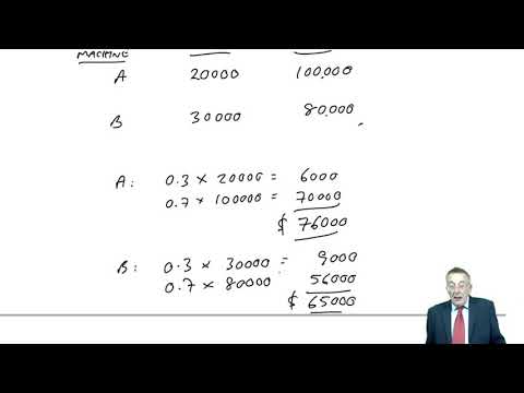
The outcome of a new venture has been forecast below.
Probability of $50,000 profit = 0.3
Probability of $(20,000) loss = 0.7
What is the expected value of this project?
Should the decision maker go ahead with the venture?
Show answerHide answer
4.1 Limitations of the expected value method
It is a long-run average applied to a short-run decision. The venture in Example 1 will be undertaken once, and $1,000 is not one of its possible outcomes.
The expected value is often an impossible result. An expected demand of 53,000 units where demand can only be 40,000, 50,000 or 60,000 is a number that will never occur.
It depends entirely on the probabilities, and in practice those are estimates. A small change in a probability can change the decision, and nothing in the technique tells you how reliable the probabilities were.
It ignores the spread of the outcomes. Two decisions with the same expected value can have completely different risk profiles — which is what the standard deviation in chapter 15 was for.
It ignores the decision-maker's attitude to risk, and so implicitly assumes risk neutrality.
5 Decision-making under uncertainty: payoff tables and decision rules
Where a choice has to be made between several courses of action and the outcome of each depends on something outside the decision-maker's control, the working starts with a payoff table.
5.1 The payoff table
A payoff table sets out the result of every combination of decision and outcome:
one row for each course of action open to the decision-maker (what is chosen);
one column for each possible state of the world (what is not chosen — demand, weather, a competitor's response);
in each cell, the profit, contribution or cost that combination produces.
Building the table is normally the longest part of the question and the part where marks are lost. Work out one or two cells carefully, find the pattern, and watch for a constraint — a capacity limit, an inventory rule — that caps some of the cells.
All four decision rules below are then read off the same table.
5.2 Expected value
Multiply each payoff in a row by the probability of its column and add: that is the expected payoff for that course of action. Choose the highest. This is the risk-neutral rule, and the only one of the four that uses the probabilities at all.
5.3 Maximax
For each course of action identify the best outcome, then choose the action with the best of those best outcomes — the maximum of the maxima. It is the rule of the risk seeker: it takes the chance of the highest possible return and accepts the risk of the lowest.
5.4 Maximin
For each course of action identify the worst outcome, then choose the action with the best of those worst outcomes — the maximum of the minima. It is the rule of the risk averter: it guarantees a floor, at the cost of giving up the chance of the highest return.
The three names look alike and the workings do not. Maximax and maximin both scan the payoff table; minimax regret needs a second table built first. Read the requirement twice before you start, because doing the right arithmetic for the wrong rule earns nothing.
5.5 Minimax regret
Maximin has an obvious weakness. If choice A returns $10 or $100 and choice B returns $9 or $10,000, maximin picks A to protect a single dollar and gives up $9,900. What that comparison is really about is not the outcome but the opportunity lost, and that is what minimax regret measures.
Take the payoff table. For each column — each state of the world — find the best payoff available in that column.
Replace every cell with the difference between that best payoff and the cell's own payoff. That is the regret: what the decision-maker gives up by having chosen this action when that state occurs. The best cell in each column becomes zero.
For each row, identify the maximum regret.
Choose the row with the smallest maximum regret — the minimum of the maxima.
Watch the direction
Regrets are losses, so the best of the worst is the SMALLEST maximum regret, not the largest. Maximin picks the largest of the minimum payoffs; minimax regret picks the smallest of the maximum regrets.
5.6 The value of perfect information
A decision-maker facing an uncertain state of the world can sometimes buy information about it — market research, a survey, a trial. The question is how much that information is worth.
Perfect information is information that is always right: if the research says demand will be 500 units, demand will be 500 units. It does not remove the uncertainty about which answer will come back — that is why it is worth buying — but once the answer arrives the best decision for that state can be taken with confidence.
For each possible state of the world, read off the payoff table the best payoff obtainable if that state were known in advance, and the action that produces it.
Weight those best payoffs by the probability of each state occurring. That is the expected value WITH perfect information.
Subtract the expected value WITHOUT perfect information — the highest expected payoff from section 5.2, because the comparison is always made on the expected value basis.
EVPI = EV with perfect information − EV without perfect information
The result is the maximum the decision-maker should pay. Pay more and the information costs more than the better decisions it enables.
The probability that the research reports a given state is the probability of that state itself — the research is perfect, so it reports what will happen. And the expected value with perfect information is not a sum the decision-maker will actually receive: one of the four payoffs will occur, not their average.
This lecture works part (c) of Example 2 and is the cleanest recording in the chapter. Keep the payoff table from the previous lecture in front of you — the tutor refers back to it throughout.

John has a factory capacity of 1,200 units per month.
Units cost him $6 each to make and his normal selling price is $11 each. However, the demand per month is uncertain and is as follows:
Demand | Probability |
400 | 0.2 |
500 | 0.3 |
700 | 0.4 |
900 | 0.1 |
He has been approached by a customer who is prepared to contract to a fixed quantity per month at a price of $9 per unit. The customer is prepared to sign a contract to purchase 300, 500, 700 or 800 units per month.
The company can vary production levels during the month up to the maximum capacity, but cannot carry forward any unsold units in inventory.
(a) Calculate all possible profits that could result from the various demand levels.
(b) Determine for what quantity John should sign the contract, under each of the following criteria:
expected value
maximin
maximax
minimax regret
(c) What is the most that John would be prepared to pay in order to obtain perfect knowledge as to the level of demand?
Show answerHide answer
6 Decision trees
A decision tree is a diagram of the alternatives open to a decision-maker and the outcomes that may follow. It is used with the expected value approach, and it earns its place when there is more than one decision to be made — particularly where a decision taken now determines what choices will be available later.
6.1 Conventions
A square is a decision point — a branch the decision-maker chooses.
A circle is an outcome point — a branch decided by something outside the decision-maker's control, with a probability on each line leaving it.
Lines run left to right from decisions and outcomes to what follows them. Probabilities and cash flows are written along the line they belong to, and the value at the end of a path is written at its right-hand end.
6.2 Rolling the tree back
Draw the tree forwards, from today's decision to the final outcomes. Evaluate it backwards, from right to left:
At each outcome point, replace the uncertainty with its expected value.
At each decision point, choose the branch with the highest value and carry that value back. Mark the branch chosen — those marks are part of the answer.
Continue leftwards until the first decision point is reached.
Deduct costs on the branch that incurs them
A cost paid to take a branch — the refurbishment, the research fee — is deducted at the point where it is committed, not at the end of the path. Roll back the expected value of what follows the branch, then subtract the cost of taking it.
This lecture builds the tree for Example 3 from a blank screen and rolls it back node by node. Two notices. The tutor labels the nodes A, B and C as he draws them; the printed answer, the figures below and the roll-back table label the same nodes 2, 3 and 1, so match them by position rather than by letter. He also rounds the cheap-refurbishment expected value of 8.095 to 8.1, which does not change any decision.

Combi plc are having problems with one of their offices and have decided that there are three courses of action available to them:
(a) shut down the office, raising proceeds of $5 million
(b) have an expensive refurbishment of the office costing $4,000,000
(c) have a cheaper refurbishment of the office at a cost of $2,000,000
If they do the expensive refurbishment, then a good result will yield a return of $13,500,000 whereas a poor result will yield a present value of only $6,500,000.
If they alternatively decide to do the cheaper refurbishment, then a good result will yield a return of $8,500,000 whereas a poor result will yield $4,000,000.
In either case, the probability of the refurbishment achieving a good result has been estimated to be 2/3.
An independent company has offered to undertake market research for them in order to identify in advance whether the result of refurbishment is likely to be good or poor. The research will cost $200,000 and there is a 68% probability that it will indicate a good result.
Unfortunately, the research cannot be guaranteed to be accurate. However, if the research indicates a good result, then the probability of the actual result being good is 91%.
If the survey indicates a poor result, then the probability of the actual result being good is 13%.
Combi have already decided that if they do have market research, and if the research indicates a poor result, then they will only be prepared to consider the cheaper refurbishment.
Use a decision tree to recommend what actions should be taken.
Show answerHide answer
7 Sensitivity analysis in decision-making
Chapter 15 used sensitivity analysis on the NPV of a capital project. The same technique applies to any decision whose outcome depends on several uncertain input variables — a product launch resting on estimated demand, selling price and variable cost, for example.
The method is unchanged. Calculate the result on the estimated figures, then, for each variable in turn and holding the others constant, calculate the percentage change that would reduce the result to break-even.
Sensitivity = (Profit ÷ Value of the item affected) × 100%
Note which figure goes underneath. For selling price it is total revenue; for sales volume it is contribution, because a change in volume moves revenue and variable cost together; for a cost it is that cost.
A short, clean recording that works Example 4 line by line and then comments on the results. It teaches the 2027 outcome correctly.

Harry is about to consider a new business opportunity. Based on his current estimations, the opportunity looks profitable.
His forecasted sales revenue is $30,000 per year — based on 1,000 units sold.
His accountant has helped him to estimate fixed costs of $15,000 per annum.
The variable costs per unit are likely to be $10 per unit.
(a) Confirm, on the basis of the above figures, that the new opportunity is worthwhile.
(b) Calculate the sensitivity to change of:
(i) sales revenue (selling price)
(ii) sales volume
(iii) total variable costs
(iv) fixed costs
(c) Comment on the results.
Show answerHide answer
8 Choosing between the techniques
Technique | Needs probabilities? | Use it when |
Expected value | Yes | The decision repeats, or the decision-maker is risk neutral and wants one number. |
Maximax | No | The decision-maker is a risk seeker, or the probabilities are not credible. |
Maximin | No | The downside must be contained — a small entity that could not survive the worst case. |
Minimax regret | No | The concern is the opportunity forgone rather than the outcome itself. |
Value of perfect information | Yes | Information about the uncertain state can be bought, and its price has to be judged. |
Decision tree | Yes | There is more than one decision, and the later ones depend on what happens first. |
Sensitivity analysis | No | The question is how wrong an estimate can be before the decision changes. |
9 Test your knowledge
Two quick checks before you move on: work through the flashcards to fix this chapter’s key terms and definitions, then sit the objective questions for exam-style practice. Both mark themselves and explain the answers as you go.
Risk and Uncertainty
12 questionsAnswer the questions one at a time. Your progress is saved so you can leave and come back.
Open chapter practice