
Pricing

1 Introduction
Selling price is one of the key decisions for anyone who trades in goods or services, and it is one the management accountant is expected to inform.
Set the price too high and demand may not be sufficient to make a profit. Set it too low and demand may exceed the capacity to supply — and the opportunity to earn a greater profit at a higher price has been given away.
Many factors influence the right price, and the particulars of each situation — the industry, the type of product, the level of competition — call for different approaches. This chapter covers the cost-based methods, the economist's model of price and demand, the profit-maximising calculation by both the tabular and the algebraic route, price elasticity, and the pricing strategies the syllabus names.
What the syllabus asks
P2B4 requires you to discuss pricing decisions for maximising profit in imperfect markets, the types of pricing strategy available, and the financial consequences of each.
"Imperfect market" is the key phrase and section 5.3 explains it. In shorthand: a market in which the seller's own price affects the quantity it can sell. Everything in sections 4 to 6 is an analysis of that case — which is why the demand curve slopes downwards rather than being a horizontal line at the market price.
2 Factors influencing selling price
Factors influencing price
Required
List as many factors as you can think of that could influence the selling price of a product.
Show answerHide answer
Most influences on price fall into three categories, sometimes called the three Cs:
The question it answers | Why it constrains the price | |
Costs | What does it cost us to make and sell? | In a normal situation the price must exceed cost if the product is to be profitable. Costs set a floor — though not always: see loss leaders and penetration pricing in section 7. |
Competitors | What are the alternatives charging, and how will they react? | If competitors sell an equivalent product for less, we must either match them or convince customers that ours is worth more. Competitors set a ceiling. |
Customers | What will customers pay, and how many will buy at each price? | For most products, the higher the price the fewer units are sold. That trade-off is the subject of sections 4 to 6. |
3 Cost-plus pricing
This recording covers sections 2 to 5.1 — the three Cs, cost-plus, the demand curve and the tabular approach — and works Examples 2, 3 and 4.
Notice one. It is in pounds in places and dollars in others; the notes are in dollars throughout.
Notice two. It reads Example 2's budgeted production as "£10,000 a year". The figure is 10,000 units a year, which is how it is used a moment later.
Its closing passage — that the tabular approach is limited to the prices the question happens to list, and that in principle the price could be dropped by one cent at a time — is the bridge to section 5.2 and is worth hearing.
Notice three. Twice it frames the pricing problem as a monopoly — “even if we were a monopoly, we're the only producers of the goods”. The syllabus's framing is wider — imperfect markets — and section 5.3 says why the distinction matters.
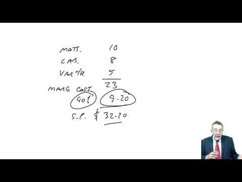
Under cost-plus pricing the selling price is built up from cost:
Selling price = Cost per unit + Profit margin
Which raises two questions: which cost, and which profit?
The profit may be added as a mark-up (a percentage of cost) or expressed as a margin (a percentage of selling price). The two are not the same and a question will tell you which it wants.
3.1 Full cost plus
Full cost includes a share of production overheads and often of non-production costs as well.
Advantages | Disadvantages |
Simple, and it ensures that all costs are covered if the budgeted volume is achieved. | The overhead absorbed per unit depends on the volume assumed — and the volume depends on the price, which is what is being calculated. The reasoning is circular. |
Useful where a business has many products and cannot appraise each price individually. | It takes no account of what customers will pay or of what competitors charge. |
It gives a defensible basis for a price in a contract negotiation, and is common in cost-plus contracts. | It can price a product out of the market when volumes fall, because the overhead per unit then rises, forcing the price up just as demand is weakening. |
3.2 Marginal cost plus
Here the price is built on the marginal (incremental) cost of producing one more unit, with a mark-up added to cover fixed costs and profit.
Advantages | Disadvantages |
It avoids the circular overhead-absorption problem entirely. | It does not guarantee that fixed costs are covered — that depends on the mark-up and on the volume actually sold. |
It is the right basis for a one-off order, or for pricing spare capacity, where the fixed costs will be incurred anyway. | Consistently used, it can lead to a general drift towards prices that are too low. |
The mark-up can be varied by product, by customer or by season without disturbing the cost base. | It gives no indication of long-run viability, because in the long run all costs are variable. |
3.3 Opportunity cost plus
A marginal cost approach that also brings in any opportunity forgone — a relevant costing approach, on exactly the principles set out in chapter 12. It is the correct basis where the order consumes a resource that is scarce, because the contribution lost on the displaced work is a genuine cost of taking this order.
Cost-plus pricing
A new product is being launched and the following costs have been estimated:
$ per unit | |
Materials | 10 |
Labour | 8 |
Variable overheads | 5 |
Fixed overheads have been estimated at $50,000 per year, and budgeted production is 10,000 units per year.
Required
Calculate the selling price based on:
full cost plus 20%;
marginal cost plus 40%.
Show answerHide answer
4 The economist's view of price and demand
Economic theory holds that, for a normal good, the higher the selling price the lower the quantity demanded. This inverse relationship is the demand curve.
The relationship is not really a straight line, but for every calculation in this chapter it is assumed to be one. On that assumption the demand curve has the equation:
P = a − bQ
where:
P is the selling price per unit;
Q is the quantity demanded at that price;
a is the theoretical maximum price — the vertical-axis intercept. At a price of a or above, demand is zero;
b is the gradient of the demand curve: the change in price divided by the change in quantity.
b = change in price ÷ change in quantity
The intercept a can be found by working back from any known price and quantity:
a = current price + ((current quantity ÷ change in quantity) × change in price)
In that formula the "change in price" is the size of the price step that causes the stated change in quantity — not the price itself, and not a percentage. If a $1 increase loses 2,500 units, the change in price is $1 and the change in quantity is 2,500.
Deriving the demand equation
A company sells an article at $12 per unit and has a demand of 16,000 units at this price.
If the selling price were increased by $1 per unit, it is estimated that demand would fall by 2,500 units.
Required
On the assumption that the price/demand relationship is linear, derive the equation relating the selling price to the demand.
Show answerHide answer
5 The profit-maximising price and output
Two methods are available, and both are examinable.
5.1 The tabular approach
Build a table from the information in the question showing costs and revenues at a range of selling prices. Once tabulated, the optimal selling price is simply the one at which total profit is highest.
It is worth adding marginal revenue and marginal cost columns even when the question does not ask for them, because they show why the profit peaks where it does — and they are the bridge to the algebraic method in 5.2.
The tabular approach
Kennedy plc has established that the price/demand relationship is as follows:
Selling price per unit $ | Demand (units) |
16.00 | 100 |
15.50 | 200 |
15.00 | 300 |
14.50 | 400 |
14.00 | 500 |
13.50 | 600 |
13.00 | 700 |
It has also established the following cost per unit of production:
Quantity (units) | Cost per unit $ |
100 | 14.0 |
200 | 13.9 |
300 | 13.8 |
400 | 13.7 |
500 | 13.6 |
600 | 13.5 |
700 | 13.4 |
800 | 13.3 |
900 | 13.2 |
Required
Complete a table using the headings below to find the optimal (profit-maximising) selling price.
Selling price p.u. | Demand | Cost p.u. | Total revenue | Total cost | Total profit | Marginal revenue | Marginal cost |
Show answerHide answer
5.2 The algebraic approach: MC = MR
This recording works Example 5 and derives the marginal revenue equation, both by differentiation and as a rule to learn. Its arithmetic is sound: MR = 300 − 0.008Q, Q = 32,500 and the price read off the demand curve at $170. One notice. It closes by saying of price elasticity: “I'm not actually going to do that … you can check the answer to the exercise at the back of the notes.” That exercise is Example 6, and its answer sits directly beneath it in section 6.

Once the price/demand relationship is known, total revenue follows from it, because total revenue is price × quantity:
TR = PQ = (a − bQ)Q = aQ − bQ2
Differentiating gives marginal revenue — the extra revenue from selling one more unit:
MR = a − 2bQ
You do not have to differentiate to use it. The rule is simply that the marginal revenue equation is the demand equation with the b term doubled.
Profit is maximised where marginal cost equals marginal revenue:
MC = MR
Marginal cost is normally the variable cost per unit. Equating the two and solving gives the profit-maximising quantity; substituting that quantity back into the demand equation — not the marginal revenue equation — gives the profit-maximising price.
Solving MC = MR gives Q, and the commonest error in the topic is to stop there, or to put that Q back into MR = a − 2bQ. The price is read off the demand curve: P = a − bQ. In the graph above, MR meets MC at a height of $40 — but the price customers pay at that quantity is $170, which is on the curve above it.
The algebraic approach
Oggi Co manufactures an item G which has an estimated demand curve of P = 300 − 0.004Q.
The variable cost of each G is $40.
Required
Use this information to find the profit-maximising selling price for one unit of G.
Show answerHide answer
5.3 Imperfect markets — what the analysis assumes
The whole of sections 4 and 5 assumes an imperfect market: one in which the seller's own price affects the quantity it can sell, so that the demand curve it faces slopes downwards.
Market | The demand curve facing one seller | The pricing decision |
Perfect competition | Horizontal at the market price — the seller can sell any quantity at that price and nothing at all above it. | There is no decision. The seller is a price taker and the only question is how much to produce. |
Imperfect market (including monopoly, oligopoly and monopolistic competition) | Downward-sloping — raising the price loses some but not all customers. | There is a real decision, and MC = MR identifies the point at which the trade-off between margin and volume is best. |
The syllabus's wording is "pricing decisions for maximising profit in imperfect markets". A monopoly is the clearest case but it is not the only one: almost any differentiated product — a brand, a location, a service with switching costs — faces a downward-sloping demand curve and can therefore use this analysis.
6 Price elasticity of demand
For a normal good a rise in price reduces demand, but by how much varies enormously between products. Price elasticity of demand measures that responsiveness:
PED = % change in quantity demanded ÷ % change in price
Both percentages are measured against the original figures. The result is conventionally quoted as a positive number, the minus sign that arises from the inverse relationship being taken as read.
Result | Name | What it means for a price cut |
PED greater than 1 | Elastic | Demand is sensitive to price. A price cut raises total revenue, because the extra volume more than compensates for the lower margin per unit. |
PED equal to 1 | Unit elastic | Total revenue is unchanged by a price change. |
PED less than 1 | Inelastic | Demand is insensitive to price. A price cut reduces total revenue — and a price rise increases it. |
Elasticity is not a fixed property of a product. On a straight-line demand curve it falls steadily as you move down the curve, which is what Example 6 demonstrates.
Price elasticity of demand
Using the figures from Example 4:
Required
Calculate the price elasticity of demand:
if the current selling price is $16 per unit;
if the current selling price is $15 per unit.
Show answerHide answer
7 Pricing strategies
This recording runs through each of the nine strategies with an illustration. It is sound, its examples are good ones, and it states the predatory-pricing legal position in full. One notice. Its illustrations are drawn from around 2019 — flat-screen televisions for market skimming, and geographical price discrimination described as “getting harder to achieve”. The mechanisms are unchanged; only the examples have aged. Section 7's table gives current-neutral illustrations.
A pricing decision is often a strategic one — to gain market share, to establish a new product, or to damage a competitor's revenues — rather than an attempt to maximise this period's profit. The syllabus names these strategies and requires you to explain each, to consider its financial consequences, and to suggest circumstances in which it is suitable.
Strategy | What it is | Financial consequence | When it is suitable |
Penetration pricing | A deliberately low initial price, sometimes below cost, with the intention of raising it once a share of the market has been won. | Low or negative margins at first, in exchange for volume and a customer base. Only worth it if the later price rise sticks. | A new entrant to an established market; where demand is elastic; where unit costs fall sharply with volume; where customers are slow to switch once they have chosen. |
Market skimming | A high initial price aimed at the customers least sensitive to price, reduced in stages as the market broadens. | High margins early, recovering development costs quickly, at the cost of low initial volume. | A genuinely new or innovative product with no close substitute; a strong brand; a short product life cycle where the money must be made early (chapter 4). |
Loss leaders | One product priced below cost to draw customers in, in the expectation that they will buy others at normal prices. | A planned loss on one line funded by the margin on the rest of the basket. It fails if customers buy only the leader. | Retailers with a wide range; products customers can price-compare easily; situations where the visit itself is what has to be won. |
Product bundling and optional extras | Several products sold together for less than the sum of their individual prices, or a base product sold cheaply with profitable extras. | Higher total revenue per customer, and it can move slow-selling lines. The margin on the bundle must be managed, not assumed. | Products that are complementary or are naturally bought together; software and subscription services; where the extras carry a much higher margin than the base. |
Product differentiation | Charging more by making the product distinguishable — through quality, features, service or brand. | A higher price supported by a real cost of differentiation. The margin gain must exceed that cost. | Markets where customers value more than price; where the difference is visible before purchase and hard for competitors to copy quickly. |
Price discrimination | Charging different prices to different customers for essentially the same product, by segment, time, location or channel. | Captures more of what each segment is willing to pay, so total revenue rises without a cost increase. | Only where the segments can be kept apart and resale between them prevented. Digital channels and price-comparison sites have made this harder, and some forms of it are legally restricted. |
Premium pricing | A permanently high price used as a signal of quality or exclusivity. | High margin on lower volume; the price itself is part of the product's appeal, so discounting damages it. | Luxury goods; markets where quality cannot be judged before purchase and price is used as a proxy for it. |
Psychological pricing | Prices set just below a round figure — $9.99 rather than $10 — or ending in particular digits. | A small revenue sacrifice for a disproportionate effect on the number of units sold. | Consumer markets and high-volume retail. Little use in business-to-business markets, where buyers are professional. |
Predatory pricing | Pricing below cost with the deliberate intention of forcing a competitor out of the market, and raising prices afterwards. | Sustained losses now, in the hope of higher prices later — a return that may never arrive. | ⚠️ Rarely, if ever, and in most jurisdictions it is unlawful as an abuse of a dominant position. Know what it is, and know that recommending it raises both a legal and an ethical problem. |
Cost-plus builds the price up from cost and ignores the customer; the economist's model starts from the customer. In an imperfect market the demand curve slopes down, P = a − bQ, and profit is maximised where MC = MR, where MR = a − 2bQ — solve for Q, then read the price off the demand curve. Elasticity is the % change in quantity over the % change in price, and it falls as you move down a straight-line demand curve. Nine named strategies, each with a financial consequence and a set of circumstances it fits — and one of them, predatory pricing, is usually unlawful.
8 Test your knowledge
Two quick checks before you move on: work through the flashcards to fix this chapter’s key terms and definitions, then sit the objective questions for exam-style practice. Both mark themselves and explain the answers as you go.
Pricing
12 questionsAnswer the questions one at a time. Your progress is saved so you can leave and come back.
Open chapter practice