
Forecasting


1 Forecasting techniques
Forecasting is important in strategic planning because a strategic plan or a budget inevitably means trying to look into the future and estimate, costs, volumes sales revenues and so on.
it is important to be able to interpret the results, use the results and be aware of where caution might be needed when relying on estimates.
Techniques covered are:
Linear regression and coefficients of determination
Time series analysis
Expected values
Decision trees
Scenario planning
2 Linear regression
Linear regression is a method of fitting the best straight line through a set of points. In business, typically the line would connect points showing:
Cost and volume
Selling price and sales volume
Hours worked and units produced
Linear regression will give constants which fit a line of the type:
y = ax + b
where:
y is the dependent variable (cost, hours, volume sold)
x is the independent variable (units made, selling price).
The constant ‘a’, for example, could be the additional cost for each additional unit made; ‘b’ would be the cost even if no units were made (the fixed cost).
3 Linear regression - caution
Be warned: linear regression will give the best line it can through any set of points. For example, if you numbered the days in the year 1 – 365 and you noted the day each person was born and the amount of money they had in their bank account, linear regression would suggest the best relationship it could between these variables.
Obviously there would not actually be a good relationship.
To test the relationship you must calculate the coefficient of correlation (r), or the coefficient of determination (r2).
r can vary between:
r = +1, meaning perfect positive correlation where all points lie on the line and as one variable increases, so does the other.
r = -1, meaning perfect negative correlation where all points lie on the line and as one variable increases, the other decreases.
r = 0 means no correlation.
If r = 0.7, r2 = 0.49 or about 50%. This means that 50% of the change in one variable is explained by the change in the other.
Caution!
You should be aware of the following before you rely on any prediction based on linear regression:
If r2 is low, then one variable is not well-associated with the other, so any predictions are liable to be poor.
The more points (readings) the better: simply more evidence for the association.
Extrapolation (predicting outside the range examined) is dangerous as we have no direct evidence of what happens in other regions. For example, costs might suddenly increase.
Other known influences (such as inflation) should be removed before the analysis.
Even good correlation does no prove cause and effect: both variables might have moved together under the influence of another variable.
4 Time series analysis - components
A time series is simply one that moves with time: sales each day, rainfall each month, machine breakdowns each week.
There are four components of a time series:
The trend – an underlying increase/decrease
Seasonal variations – regular variations with a cycle length of less than a year.
Cyclical variations – regular variations with a cycle length of more than a year
Random variations – irregular and unpredictable.
Time series analysis tries to analyse the first two of these.
The figure below shows a rising trend with regular seasonal variations.
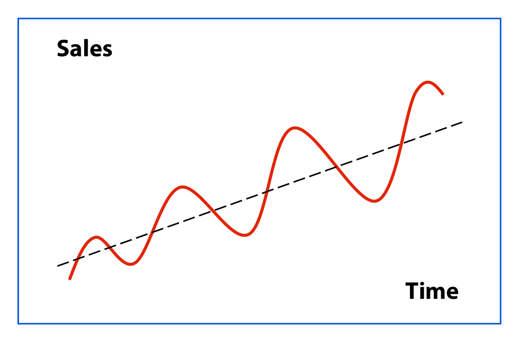
There are statistical techniques for isolating estimated of the trend and each of the seasonal variations. In some situations this will result in more accurate forecasts than linear regression, which cannot take into account seasonal variations and always produces a straight line.
5 Expected values
Project 1 | p | Income $ | p x Result | Project 2 | p | Income $ | p x Result |
Outcome 1 | 0.5 | 1,000 | 500 | Outcome 1 | 0.5 | 5,000 | 2,500 |
Outcome 2 | 0.5 | 11,000 | 5,500 | Outcome 2 | 0.5 | 7,000 | 3,500 |
Expected value | 6,000 | Expected value | 6,000 |
The expected value is the sum of the outcomes weighted by the probability of them occurring.
Expected values have two main problems (apart from estimating the probabilities):
The expected value is not usually ‘expected’ in once-off projects. neither project above actually predicts $6,000
The expected value does not give any information about risk. For example, in Project 1 above there is a huge difference between the two outcomes and, in particular, a very large downside risk where only 1000 of income is received, and that could be very serious for the firm. Project 2 is much safer, with a worse case expected of $5,000.
6 Decision trees - example
Decision trees allow more complex projects and decisions to be mapped out.
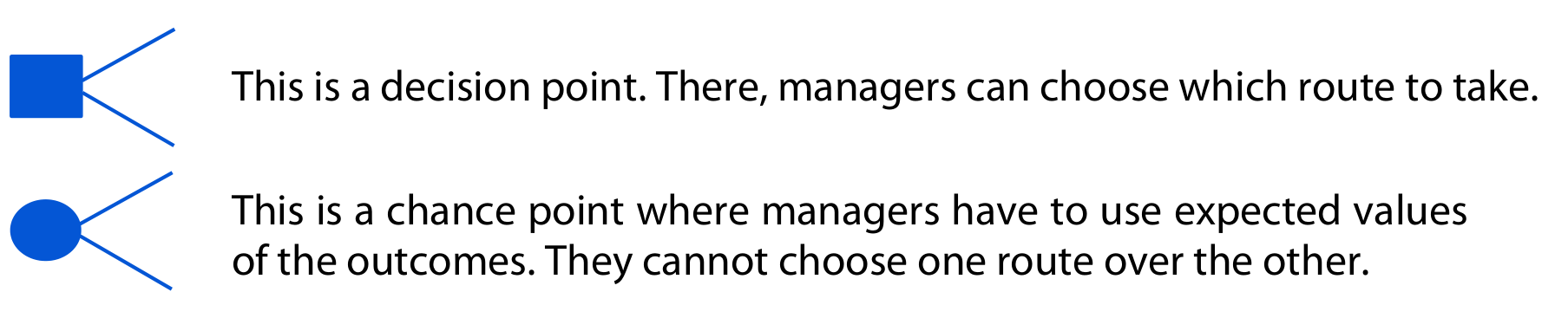
The technique uses two symbols:
For example:
A project initially costs $5 million and income for the first year will be $3 million with a probability of 0.6 and an income of $2 million with a probability of 0.4.
At the end of the second year the project could be upgraded for $2.5 million and then income would be $6 million with a probability of 0.7 or $3 million with a probability of 0.3.
If the project were not upgraded, the year one income, whatever it had been, would repeat in year two.
7 Decision trees - solution
The project can be represented by the following diagram.
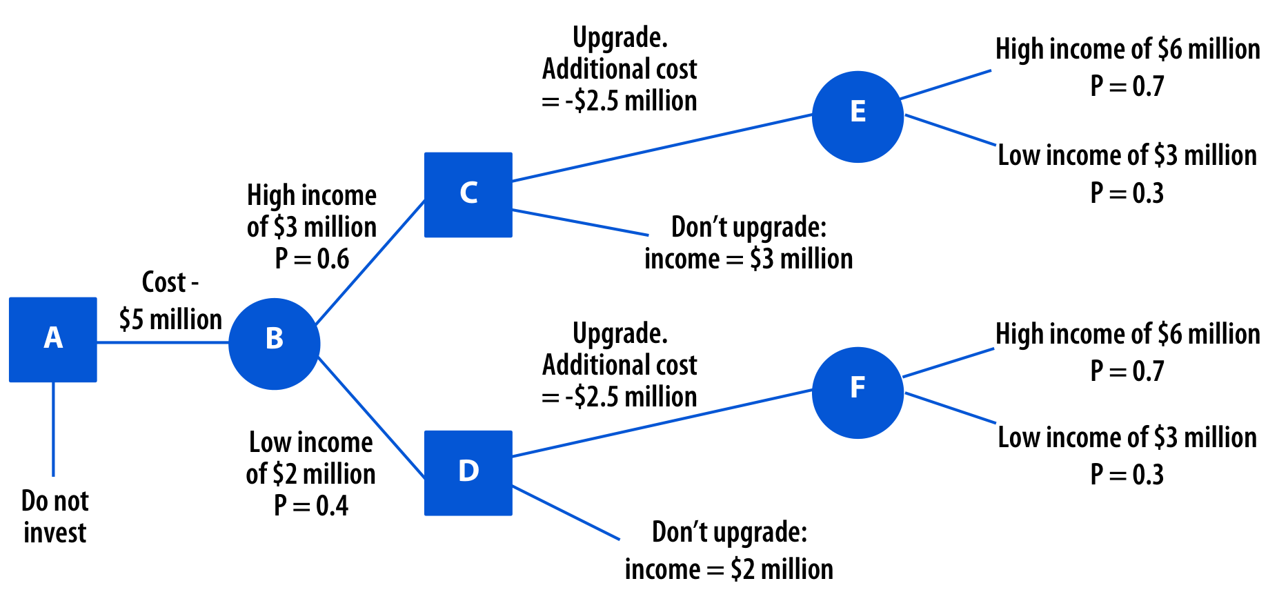
Having drawn the diagram, you then go to the right hand side and begin to ‘roll-back’ through the decisions and chance points.
Expected value at E = 0.7 x 6 + 0.3 x 3 = $5.1 million
Value at C is therefore:
5.1 – 2.5 = $2.6 million or $3 million. Therefore the decision at C should be not to upgrade.
Expected value at F is $5.1 million (as for point E)
Value at D is therefore:
5.1 – 2.5 = $2.6 million or $2 million. Therefore the decision at D should be to upgrade.
Expected value at B is: 0.6 x (3 + 3) + 0.4 x (2 + 2.6) = 5.44
Value at A is therefore 5.44 – 5 = 0.44 or $Nil, if nothing done.
Therefore, start the project. If there is high income in year 1, do not upgrade for year 2. If there is low income in year 1 then do upgrade for year 2.
8 Scenario planning
You will remember that earlier we used tools like PESTEL to help us to identify events that might occur and affect our organisation. Of course, many of the events are not certain, but we should be aware that, for example, interest rates might change, competitors might become more aggressive, a new product is licensed or a government might change. There are therefore many permutations of events that could occur and we need to try to make sense of those.
Scenario planning attempts to take into account all the things that could happen and from those to build a number of believable, alternative futures. Not all the events that could happen are likely to happen together. For example, if the government changes than we could predict that perhaps, interest rates would rise. In which case there is no point examining a scenario of new government and low interest rate – that is an implausible scenario. This greatly helps to reduce the number of ‘universes’ we have to consider and allows the organisation to concentrate on the few most likely ones.
Interest rate = 3% | Interest rate = 7% | |
Government 1 | Implausible combination | Scenario 1 |
Government 2 | Scenario 2 | Implausible combination |
Here, the organisation would concentrate on what its response should be to each of the plausible scenarios.