
Risk and Uncertainty

1 Introduction
A major reservation of any investment appraisal decision is that the figures used in the calculations are only estimates and stand to be uncertain. Clearly if any of the cash flows used in the decision turn out to be different from what was estimated, the decision itself could be affected.
In this chapter we will revise three approaches that you should already be aware of from the earlier Financial Management exam, and then look at one more approach - Value at Risk.
2 Sensitivity analysis
Sensitivity analysis analyses the effect of changes made to variables in the problem in order to determine their effect on the decision.
First we calculate the NPV of the project on the basis of the best estimates.
Then we calculate what % change (or sensitivity) in each of the variables would result in a NPV of zero (i.e. the breakeven position – any further change would change the decision).
By considering the sensitivity of each variable we can ascertain which variables are the most critical and therefore perhaps need more work confirming our estimates.
When a requirement asks you to discuss the assumptions behind an NPV, writing that sensitivity analysis should be carried out earns little on its own. Say what it would show — the percentage change in each key estimate that would bring the NPV to zero, and so which estimates the decision depends on most and most need checking — and note its limit: it changes one variable at a time.
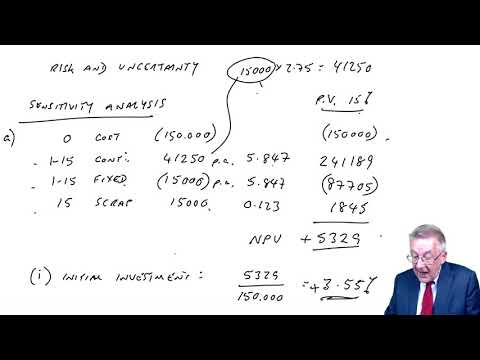
Daina has just set up a new company and estimates that the cost of capital is 15%.
Her first project involves investing in $150,000 of equipment with a life of 15 years and a final scrap value of $15,000.
The equipment will produce 15,000 units p.a. generating a contribution of $2.75 each. She estimates that additional fixed costs will be $15,000 p.a..
Determine, on the basis of the above figures, whether the project is worthwhile
Calculate the sensitivity to change of:
the initial investment
the sales volume p.a
the contribution p.u.
the fixed costs p.a.
the scrap value
Comment on the results
Show answerHide answer
3 Simulation
Simulation is a technique which allows more than one variable to change at the same time.
You will not be required in the examination to actually perform a simulation, but you should be aware of the principle involved.
Essentially, the stages are as follows:
identify the major variables
specify the relationship between the variables
attach probability distributions to each variable and assign random numbers to reflect the distribution
simulate the environment by generating random numbers
record the outcome of each simulation
repeat the simulation many times to be able to obtain a probability distribution of the possible outcomes
4 Expected values
With this approach, we identify the various possible outcomes for each uncertain variable, together with the associated probability.
We then use for each uncertain variable the weighted average outcome (or expected outcome), and use these figures in our investment appraisal calculation.
Daiga plc is considering launching a new product.
This will require additional capital investment of $200,000.
The selling price of the product will be $10 p.u.. Daiga has ascertained that the probability of a demand of 50,000 units p.a. is 0.5, with a probability of 0.4 that it will be 20% higher, and a 0.1 probability that it will be 20% lower.
The company expects to earn a contribution of 50% and expects fixed overheads to increase by $140,000 per year.
The time horizon for appraisal is 4 years. The machine will be sold at the end of 4 years for $50,000.
The cost of capital is 20% p.a.
Calculate the expected NPV of the project
Show answerHide answer
5 Value at Risk (VaR)

When we calculate the NPV of a project, the problem is, of course, that the cash flows are uncertain and that therefore the actual NPV may turn out to be higher or lower. We have looked at the sensitivity - the % changes that will result in an NPV of zero. However, Value at Risk is a method of calculating with a certain degree of confidence what the greatest fall in the NPV will be.
The VaR is the maximum amount that an investment might lose at a given level of confidence. For example, we might be able to say that the VaR is $100,000 at the 95% confidence level. This would mean that there would be only a 5% chance of losing more than $100,000.
Although we are able to calculate the VaR for a project, it is much more applicable to an institution (for example a bank) holding a portfolio of investments. The current value may be, say, $500,000, and obviously the value may increase or decrease over time. It will be of use to the bank to be able to calculate that they are 95% confident that the value will not fall by more than $300,000 (i.e. to less than $200,000) so as to be able gauge the amount of assets needed to be able to cover possible losses.
In order to be able to calculate the VaR, we need to know the volatility of the values (the standard deviation) and to assume that they values are normally distributed. We will explain the calculation with an example.
James has estimated an annual standard deviation of $750,000 on one of its projects, based on a normal distribution of returns. The average annual return is $2,400,000.
Estimate the value at risk (VAR) at a 95% confidence level for one year, and also over the project’s life of six years.