Advanced Variances

1 Introduction

This chapter looks at variances in more detail. It builds directly on the techniques and principles of the basic variances in the previous chapter, and everything here assumes you are comfortable with those.

Planning and operational variances let management concentrate on what is controllable, by stripping out the effect of a standard that was wrong or has become out of date. That is the main topic of the chapter.

The chapter closes with activity based costing variances — the same variance thinking applied to an overhead absorbed on a cost driver rather than on a labour hour.

Scope

The 2027 syllabus outcome these variances sit near is A3c, “Variance analysis (without mix and yield variance)”, whose named topics are price and rate variances, usage and efficiency variances, and interpretation of variances. Those are the whole of chapter 9.

Planning and operational variances and ABC variances are not in that topic list. They are taught here as an extension of it — they use no technique chapter 9 did not give you, and they are the natural answer to the question chapter 9 §5 ends on: what do you do when the standard itself is the problem? Sales mix and sales quantity variances are a different matter and are dealt with in section 3.

2 Planning and operational variances

This lecture works both of the chapter's planning and operational examples in full and is the best teaching in it — Example 1's $38,500 (A) planning variance and $22,800 (F) operational, Example 2's $36,000 (A) and $33,000 (F), all of which agree with the answers below. Two points before you play it. It refers back to the basic materials and labour variances as “chapter 7”; under the current numbering that is chapter 9, because the recording was cut for an earlier edition of P1 in which basic variances came seventh. And where it says you cannot add the two rate variances together and reconcile them, it is right as far as it goes: the rate planning and rate operational variances alone do not add back to the basic rate variance. The technique does reconcile once the operational efficiency variance at the revised rate is brought in, and §2.4 below closes both examples that way.

YouTube video

2.1 Why a variance is split this way

Variance analysis helps management exercise control by identifying where there may be operational problems. But among the possible reasons for a variance is that the factor driving it was uncontrollable, or external to the entity altogether.

An adverse material price variance would normally be treated as the responsibility of the purchasing department. Suppose, though, that the increase in the material price was caused by a worldwide shortage. That is not within the purchasing manager’s control, and with hindsight the original budget should have allowed for a higher price. As it stands, the budget is built on a standard that is simply wrong.

Comparing actual results with an invalid budget tells management very little. So the results are compared with a revised budget instead, and the difference between the original budget and the revised budget is reported separately.

2.2 The two variances

Ex ante and ex post

The ex ante standard is the original standard — the one set before the period began. The ex post standard is the revised standard — the one that, with hindsight, should have been set. The revision uses only information that could not reasonably have been known at the time.

Variance	Compares	What it measures	Controllable?
Planning	original budget (ex ante) with revised budget (ex post)	the effect of the standard having been wrong	No — it measures the quality of the planning
Operational	revised budget (ex post) with actual results	performance against a standard that is now fair	Yes — this is the manager’s performance

Operational variances are the ones management acts on, because they are the ones the business can do something about. Planning variances are not ignored, however: a large planning variance is a signal that the standards themselves need revising for future periods, and it may prompt a change of plan — different suppliers, a different grade of labour, a different production method.

There is more than one way of splitting these variances, and different textbooks give different answers. The method used here is CIMA’s preferred method, as set out in the examiner’s article, and it is the one to use in the exam. If you have met this topic elsewhere and got a different answer, that is why.

In this method the planning variance is calculated on the standard quantity for the actual output, and the operational variance on the actual quantity. The two price variances therefore do NOT add up to the basic price variance on their own — the balance sits in the operational usage or efficiency variance. Section 2.4 shows the full reconciliation.

2.3 Two worked examples

Original budget

Standard labour cost per unit	$7.00
Each unit takes 0.5 hours at a labour rate of	$14.00 per hour
Budgeted production for January	20,000 units

Actual results

Production	22,000 units
Labour worked	11,400 hours
Actual labour rate	$15.50 per hour

Since the budget was prepared, the prevailing external labour rate has risen to $17.50 per hour.

Required

Calculate the labour rate planning variance and the labour rate operational variance.

Labour rate PLANNING variance — actual output × revised standard hours, at the original rate against the revised rate.

	$
22,000 units × 0.5 hrs × $14.00 (original rate)	154,000
22,000 units × 0.5 hrs × $17.50 (revised rate)	192,500
Labour rate planning variance	38,500 (A)

It is adverse because the standard has been revised upwards: with hindsight, this output was always going to cost more than the original budget allowed. Nothing the production manager could have done would have avoided it.

Labour rate OPERATIONAL variance — actual hours worked, at the revised rate against the rate actually paid.

	$
11,400 hours × $17.50 (revised rate)	199,500
11,400 hours × $15.50 (actual rate)	176,700
Labour rate operational variance	22,800 (F)

It is favourable, and this is the figure the manager should be judged on: against the rate the market was actually charging, labour was obtained for $2 an hour less.

Reading the two together. Judged against the original standard the manager looks very poor — $15.50 paid against a $14.00 standard. Split properly, the picture reverses: the entity lost $38,500 to a market movement nobody controlled, and the manager saved $22,800 against the market.

2.4 Reconciling back to the basic variance

The two variances above are both rate variances, and they do not on their own explain the whole difference between what the labour cost and what it should have cost. The missing piece is the operational efficiency variance, valued at the revised rate.

Example 1 — full reconciliation	$
Total labour cost variance: 11,400 × $15.50 = 176,700, against the original standard cost of the actual output, 22,000 × $7 = 154,000	22,700 (A)
Rate planning variance	(38,500) (A)
Rate operational variance	22,800 (F)
Efficiency operational variance: (22,000 × 0.5 = 11,000 standard hours − 11,400 actual hours) = 400 hours × $17.50 revised rate	(7,000) (A)
Total	(22,700) (A)

Note that the operational efficiency variance is valued at the revised rate of $17.50, not the original $14.00. Once the standard has been revised, every operational variance is measured against the revised standard — that is the whole point of revising it.

Original budget

Budgeted production	21,000 units
Standard material cost per unit	3 kg at $4.00 per kg

Actual results

Production	10,000 units
Materials purchased and used	33,000 kg at $4.20 per kg

A global shortage meant that the external price for this material was higher than budgeted, and should have been $5.20 per kg.

Required

Calculate the planning and the operational material price variances.

Material price PLANNING variance — actual output × standard usage, at the original price against the revised price.

	$
10,000 units × 3 kg × $4.00 (original price)	120,000
10,000 units × 3 kg × $5.20 (revised price)	156,000
Material price planning variance	36,000 (A)

Material price OPERATIONAL variance — actual quantity purchased, at the revised price against the price actually paid.

	$
33,000 kg × $5.20 (revised price)	171,600
33,000 kg × $4.20 (actual price)	138,600
Material price operational variance	33,000 (F)

Once the world price had moved to $5.20 the buyer was expected to pay $5.20; $4.20 was paid, so on the revised standard the buying was very good indeed.

Full reconciliation (not required by the question, but it is the check to make):

	$
Total materials cost variance: 33,000 × $4.20 = 138,600, against the original standard cost of the actual output, 10,000 × $12 = 120,000	18,600 (A)
Price planning variance	(36,000) (A)
Price operational variance	33,000 (F)
Usage operational variance: (10,000 × 3 = 30,000 standard kg − 33,000 actual kg) = 3,000 kg × $5.20 revised price	(15,600) (A)
Total	(18,600) (A)

The interpretation matters more than the arithmetic here. The entity spent $18,600 more on material than the original standard allowed. Almost twice that — $36,000 — was lost to a world price movement nobody could control. Against the price the market was actually asking, the buyer saved $33,000. What did go wrong operationally was usage: 3,000 kg more than the output needed, costing $15,600 at the price now ruling. Report the original $18,600 adverse figure alone and management chases the wrong manager.

2.5 The limits of the technique

REVISING THE STANDARD IS A JUDGEMENT, and the manager whose performance is being measured often has an interest in the answer. There is an obvious temptation to reclassify a poor operational result as a planning problem.
THE REVISED STANDARD MUST USE ONLY INFORMATION THAT COULD NOT REASONABLY HAVE BEEN KNOWN when the budget was set. Something that was foreseeable is a planning failure that the entity IS responsible for, even though it is reported as a planning variance.
IT TAKES TIME AND COSTS MONEY. Recalculating standards after the event is only worth doing where the amounts are large enough to change a decision.
A LARGE PLANNING VARIANCE IS ITSELF INFORMATION. If it recurs, it means the standard-setting process is not good enough, and the answer is to fix the standards rather than to keep reporting the variance.

3 Mix and yield variances — and why they are not in P1

Not examinable in P1

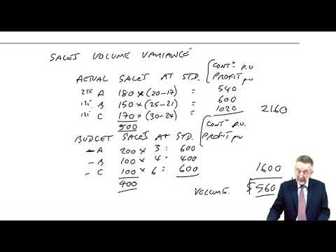
Mix and yield variances are examined at P2, not at P1: the P1 syllabus outcome A3c reads, in terms, “Variance analysis (without mix and yield variance)”. Sales mix and sales quantity variances, which analyse the sales volume variance of a multi-product business, belong to the same family and are outside P1 for the same reason.

They are named here only so that a student who meets the term knows where it belongs; nothing in P1 requires them, and no question in this chapter uses them.

The lecture below is out of P1 scope. “Sales Mix Variances” teaches sales mix and sales quantity variances correctly — the arithmetic in it was checked and it is right — but the topic is P2 material, inherited from the ACCA Performance Management syllabus this recording was originally cut for. Watch it for interest or for P2; do not spend P1 revision time on it. The recording also refers to “paper F2” at several points, which is the ACCA paper it came from, not CIMA F2.

YouTube video

4 Activity based costing variances

Eleven minutes on activity based costing variances, and it is correct throughout: a standard cost of $60 a despatch, an expenditure variance of $5,280 (F), an efficiency variance of $6,000 (A), and the two netting back to the total of $720 (A). Two of its references belong to a different paper. The example it works is Example 3 of this chapter, not the “example 6” it is called on tape, and activity based costing is chapter 4 here, not “the very first chapter” — this is a re-cut of an ACCA Performance Management master. Take its remark that the topic “was only been asked once” the same way: that is another qualification's exam history, not P1's. What is true for P1 is in the scope widget at §1 — ABC variances are not in the A3c topic list and are taught here as an extension.

YouTube video

Activity based costing, from chapter 4, allocates an overhead to products using a cost driver rather than a labour hour or a machine hour. The point of doing so is not only to encourage a cut in the total overhead but to encourage more efficient use of whatever drives it.

Suppose the despatch overhead is $100,000 for 5,000 despatches — $20 per despatch. That cost per despatch can be reduced either by cutting the total cost, which is an expenditure question, or by making fewer despatches for the same output, which is an efficiency question. The two variances are exactly the ones you already know; only the unit changes, from an hour or a kilogram to a despatch.

Variance	Compare	with
Total	actual total overhead	standard cost of the actual production
Expenditure	actual total overhead	actual number of driver units × standard cost per driver unit
Efficiency	actual number of driver units	standard number of driver units for the actual production; difference × standard cost per driver unit

Compare that table with the materials price and usage variances in chapter 9 §3.2. It is the same pair: one variance asks whether the right price was paid per driver unit, the other asks whether the right number of driver units was consumed for the output achieved. There is no new rule to learn.

The following information is available for a period:

	Budget	Actual
Production	48,000 units	50,400 units
Activity level	2,000 despatches	2,200 despatches
Total overhead cost of despatching	$120,000	$126,720

Required

Calculate the total overhead variance for despatching, and analyse it into the expenditure and efficiency variances.

Standard cost per despatch = $120,000 ÷ 2,000 = $60. Standard despatches per unit = 2,000 ÷ 48,000, so the standard cost per unit of output is $120,000 ÷ 48,000 = $2.50.

Total variance	$
Actual total expenditure	126,720
Standard cost of the actual production (50,400 units × $2.50)	126,000
Total despatch overhead variance	720 (A)

Expenditure variance	$
Actual total expenditure	126,720
Actual despatches at standard cost (2,200 × $60)	132,000
Expenditure variance	5,280 (F)

Efficiency variance	Despatches
Actual number of despatches	2,200
Standard number for the actual production (50,400 × 2,000 ÷ 48,000)	2,100
Difference	100 (A)
At the standard cost of $60 per despatch	$6,000 (A)

Check: $5,280 (F) − $6,000 (A) = $720 (A), the total variance.

Interpretation. The two tell opposite stories and both matter. Each despatch cost less than the $60 standard — a saving of $5,280. But 100 more despatches were made than the output needed, costing $6,000, and on balance the entity is $720 worse off. Under a traditional absorption system, where the despatch overhead would have been spread over labour hours, neither effect would have been visible at all. That is the argument for ABC variances: they report on the thing that actually drives the cost.

5 Test your knowledge

Two quick checks before you move on: work through the flashcards to fix this chapter’s key terms and definitions, then sit the objective questions for exam-style practice. Both mark themselves and explain the answers as you go.

Answer the questions one at a time. Your progress is saved so you can leave and come back.

Open chapter practice