More variance analysis

1 Introduction

In this chapter we will look more at variances and several ways of making them more useful to management.

Planning and Operational variances involve further analysis of the variances to assist management in deciding where more investigation should be focussed; whereas Mix and Yield variances looks at a specific situation where conventional variances might be misleading; and finally we will take another look at labour idle time variables.

2 Planning and Operational variances

YouTube videoLoad YouTube video

YouTube videoLoad YouTube video

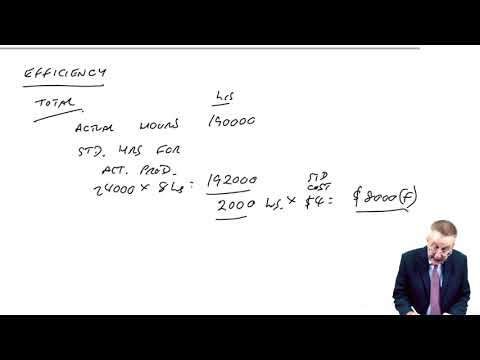
We discussed in the previous chapter that the purpose of variance analysis is to assist management in exercising control by identifying areas where perhaps there are operational problems.

We also discussed possible reasons for variances. Although these included factors such as inefficiency of the workforce – a factor that perhaps may be controlled for the future – they also included factors such as an increase in raw material prices and an incorrect standard having been used in the budgets. These last two are examples of factors that certainly can not be controlled and where it would be silly to waste time re-investigating each month. It would make more sense to compare actual results with a standard that reflects any changed conditions and is therefore realistic.

2.1 Planning variance (or revision variance)

This is a classification of variances calculated by comparing the original budget (or ex ante budget) to a budget revised for any permanent changes to a more realistic budget (ex post budget).

2.2 Operational variance

This is a classification of variances calculated by comparing actual performance with a revised (or ex post) budget. These variances are worth investigating more as they are variances caused by operating factors that potentially might be controllable.

3 Mix and Yield variances

YouTube videoLoad YouTube video

It is quite common in practice for one product to use several different materials.

For example, a desk may use wood for the top and metal for the legs.

For each of the materials we can calculate price and usage variances in the normal way, and usually this is sufficient for our purpose.

However, suppose we were manufacturing a mixed fruit juice that contained a mixture of strawberry juice and banana juice. To calculate usage variances for each material separately would be of little use – if we used less strawberry juice than budgeted, we would automatically use more banana juice. We would therefore end up with one variance favourable and one adverse, and yet the overall effect on costs could be either favourable or adverse depending on which juice was the most expensive.

In this situation, when the materials may be substituted for each other (or are substitutable) then we look at all the materials together and analyse the usage variance into the following variances:

• mix variance

  this shows the effect of changing the proportions of the mix of materials input into the process

• yield variance

  this shows the difference between the actual and expected output or yield from the process

3.1 Other mix variances

YouTube videoLoad YouTube video

Although the calculation of mix variances most commonly relates to materials, exactly the same sort of situation could be relevant for labour if there were more than one grade (paid at different rates) that were substitutable.

The approach would be exactly the same as for materials.

Slightly less obvious (although essentially the same approach) is the situation where sales are ‘substitutable’.

For example, suppose a company sold two types of desk which although similar had different profit margins. Clearly the company would hope for higher sales, but they would also be interested in the mix of sales – it would be better if customers bought more of the desks giving higher profit p.u., even if it were to mean selling fewer of the desks that gave lower profit p.u..

Again, in this situation, the approach used for materials may be useful.

4 Advanced Idle Time variances

YouTube videoLoad YouTube video

When we looked at labour variances in the previous chapter, we said that any difference between the hours paid and the hours worked was Idle Time.

However, since there is likely to be some idle time in almost every business, it would be more sensible to build some idle time into the budget and then an idle time variance would only occur if the actual idle time were more or less than budgeted.

We will look at the ‘rules’ with an example.

5 Activity Based Costing Variances

YouTube videoLoad YouTube video

You will remember from an earlier chapter that ABC is a way of allocating overheads to products using cost drivers.

The main reason for doing this was not just to encourage cutting the total cost of the overhead, but also to encourage more efficient use of the overhead.

For example, we may have had an overhead cost for despatch of $100,000 and a total of 5,000 despatches. This would mean that it was costing $20 per despatch. We could reduce the cost per despatch by either cutting the total cost (an expenditure variance) or by increasing the number of despatches (an efficiency variance).

6 The application of standard costing (and variance analysis) in the modern environment.

Modern management places great emphasis on quality - Total Quality Management (TQM), and on increasing efficiency and reducing waste - Just In Time (JIT).

However, traditional standard costing tends to make allowances for waste and for idle time, which is contrary to the TQM and JIT culture.

Traditional variance analysis focuses on quantity rather than quality. This could mean, for example, using lower quality material to save money. This would again be contrary to the TQM and JIT culture.

Another element of the TQM culture is the idea of trying to achieve continuous improvement. Traditional variance analysis does not really accommodate this.