
Analytical techniques in budgeting and forecasting

1 Introduction
In this chapter we will look at two numerical techniques that can be useful in the preparation of budgets.
One is the high-low method of cost estimation, which should be revision from Paper MA. The other is something known as learning curves.
Time series analysis and Regression analysis are two topic that are assumed knowledge from Paper MA. Although you cannot expect detailed calculations on these areas in the Paper PM exam, if you have forgotten these areas then you should watch the relevant Paper MA lectures to remind yourself - they are the lectures covering Chapters 19 and 20 of our free Paper MA lecture notes.
2 High-low method

We assume always that there are two types of costs – variable costs and fixed costs.
In practice, there are many costs which are semi-variable, i.e. part of the cost is fixed and part variable.
For budgeting purposes it is important to identify the variable and the fixed elements.
The high-low method is a very quick and simple approach to identifying the variable and fixed elements of costs.
This approach assumes that there is a linear relationship and uses just the highest and lowest observations in order to calculate the costs.
The following table shows the number of units produced each month and the total cost incurred:
Units | Cost | |
January | 100 | 40,000 |
February | 400 | 65,000 |
March | 200 | 45,000 |
April | 700 | 85,000 |
May | 600 | 70,000 |
June | 500 | 70,000 |
July | 300 | 50,000 |
Estimate the variable cost per unit, and the fixed cost per month
This approach is very simplistic. It assumes that the relationship is perfectly linear.
3 Learning curves
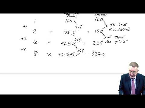

The high-low method assumes that the total variable cost is reasonably linear – that the variable cost per unit is fixed.
In the case of labour, this is very often not the case in the early stages of a new product. If we were intending to start production of a new product, then the obvious thing to do would be to produce a prototype in order to assess how long it would take to produce each unit. However, this would be dangerous because as we were to produce more and more units it is likely that the time taken for each unit would reduce as the workers gained experience. This reduction in time per unit is known as the learning effect.
3.1 Conditions
The theory of learning curves will only hold if the following conditions apply:
There is a significant manual element in the task being considered.
The task must be repetitive.
Production must be at an early stage so that there is room for improvement.
There must be consistency in the workforce.
There must not be extensive breaks in production, or workers will ‘forget’ the skill.
Workforce is motivated.
3.2 Theory
As cumulative output doubles, the cumulative average time per unit falls to a given percentage of the previous average time per unit.
Questions often ask for the learning rate itself. Where the output given doubles — the first batch and the first two, or two batches and four — no formula is needed: divide the cumulative average time per batch by the previous cumulative average. Keep the algebraic formula for outputs that are not doublings.
The time taken to produce the first unit is 100 hours.
There is a learning rate of 75%.
How long will it take to produce an additional 7 units?
3.3 Steady State
Eventually, the time per unit will reach a steady state where no further improvement can be
made.
3.4 Cessation of learning effect
Practical reasons for the learning effect to cease are:
(a) When machine efficiency restricts any further improvement
(b) The workforce reach their physical limits
(c) If there is a ‘go-slow’ agreement among the workforce
3.5 Formula
y = axb
where
y = cumulative average time per unit
x = cumulative output
a = time taken for 1st
b = a learning factor which is given by the formula:
log r ÷ log 2
r = learning rate expressed as a %.
Flogel Ltd has just produced the first full batch of a new product taking 200 hours.
Flogel has a learning curve effect of 85%.
How long will it take to produce the next 15 batches?
Flogel expects that after the 30th batch has been produced, the learning effect will cease.
From the 31st batch onwards, each batch will take the same time as the 30th batch.
What time per batch should be budgeted?
Quantitative analysis in budgeting (learning curves)
8 questionsAnswer the questions one at a time. Your progress is saved so you can leave and come back.
Open chapter practice