Microeconomics

1 Introduction

YouTube videoPlay video

Deals with the price and cost of manufacturing of goods, and with the reactions of suppliers of customers.

2 The demand curve

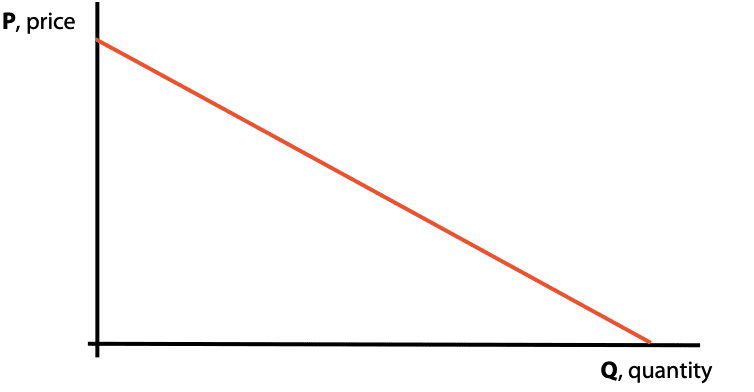
For most goods, as price increases the quantity demanded will reduce. This diagram shows a linear decrease; in practice the demand curve is likely to be curved.

The position and slope of the demand curve depend on:

• Price of goods

• Consumers’ income. Very high income might imply that a change in price will not make much difference to demand.

• Substitutes and complements. A substitute product is one that can be bought as an alternative. For example, olive oil and sunflower oil are substitutes for some purposes. If the price of olive oil increases, the demand to sunflower oil is likely to increase as consumers switch. Complementary products are often bought together. For example, cars and petrol. If the price of cars reduces, more are bought, but more petrol will also be bought even though its price has not changed.

• Fashion and taste. A fashionable item will have high demand and consumers may be prepared to pay a high price.

• Whether the goods are essential or luxury. If goods are essentials (like basic food) then higher prices will not affect demand greatly. If goods are luxuries (or at least purchase of them is discretionary), then a rise in price can cause a steep fall in demand. For example, the purchase of foreign holidays is markedly affected by the price of those holidays.

• Expectation of future price changes. If consumers think the price will rise, then current demand is increased as they stock-up on the goods.

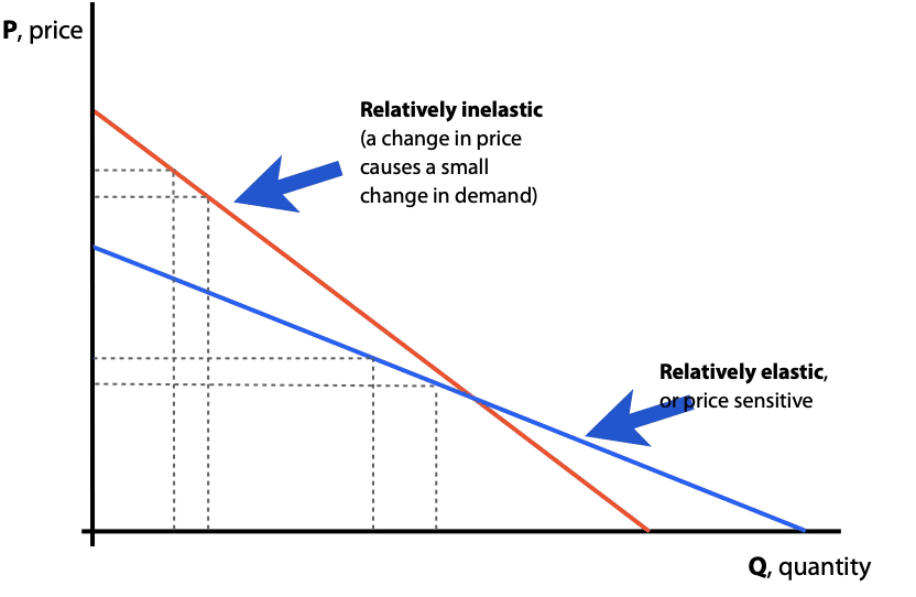
If demand is elastic, then demand for the good is price sensitive and a small change in price will cause a relatively large change in demand. That is shown by the less steep line above.

If demand is inelastic, then demand for the good is relatively price insensitive and a change in price will have a relatively small effect on demand.

Because an increase in price will normally cause a decrease in demand, technically this measure is negative, but the negative sign is usually ignored.

Price elasticity of demand >1 means that a relatively small change in price will cause a relatively large change in demand, so demand is elastic.

This has the consequent that revenue will increase if prices are reduced because the increase in demand more than compensates for the fall in price.

0 < price elasticity of demand < 1 means that a relatively small change in price will cause a relatively small change in demand, so demand is inelastic.

This has the consequent that revenue will decrease if prices are reduced because the increase in demand will not compensate for the fall in price.

Price elasticity of demand = 1 means that revenue will be constant if the price is changed slightly.

3 Calculation of the price elasticity of demand

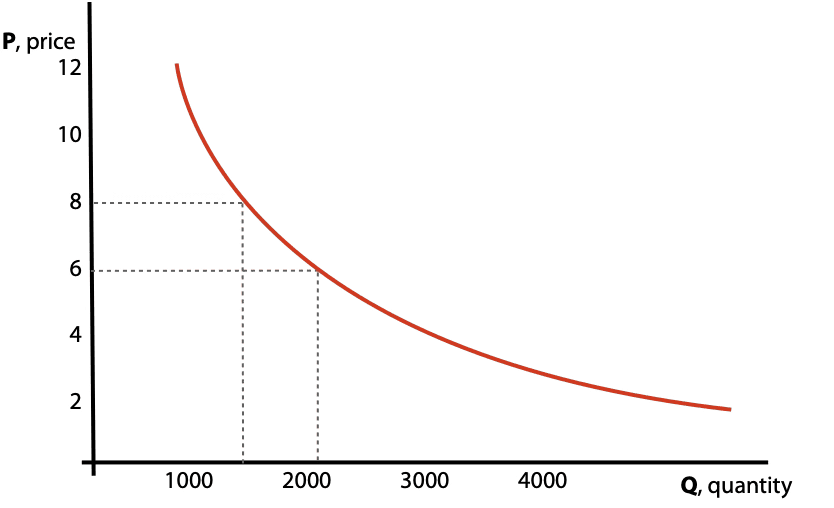
In the above diagram, say that at a price of $8, demand is 1,200 and that at a price of 6, demand is 2,200.

There are two approaches to calculating the elasticity:

Arc elasticity uses the mid point of the two quantities and prices as the basis point ie 1,700 ( = (2,200 + 1,200)/2) for quantity and 7 for price.

Proportional change in demand = (2,200 – 1,200)/1700 = 0.588 or 58.8%

Proportional change in price = (8 – 6)/7 = 0.286 or 28.6%

Price elasticity of demand = 58.8/28.6 = 2

Point elasticity uses the starting points eg start price at 8 and demand at 1,200

Proportional change in demand = (2,200 – 1,200)/1200 = 0.833 or 83.3%

Proportional change in price = (8 – 6)/8 = 0.25 or 25%

Price elasticity of demand = 83.3/25 = 3.3

Note that elasticity of demand change constantly along a demand curve, even if the demand curve is a straight line. For example, in the table below, demand increases by 1,000 units for each $1 decrease in price:

The arc price elastic of demand from $12 to $11 is:

The arc elasticity of demand between $3 and $2 is:

3.1 Income elasticity of demand

This measures how demand varies with income:

The change in demand is represented by a shift in the demand curve: same quantity demanded at a higher price or higher quantity demanded at the same price.

If the income elasticity of demand is negative then the goods are known as inferior goods because as income rises consumers change to better brands. For example, changing from inter-city bus services (cheap, but slow) to intercity trains (more expensive but faster).

Inelastic: 0 – 1: necessities. The goods were bought even when income was low.

Elastic: >1: luxuries. More goods are bought when there is ‘spare’ income.

4 Demand and supply curves

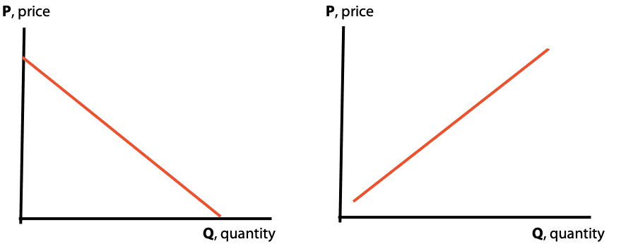
In the demand curve as the price increases, demand falls off. In the supply curve, as the price increases, production will increase because higher prices mean that there is the opportunity of more profits.

However, profits will only be made if the goods produced actually sell and an equilibrium point will be reached at a price where demand is matched by supply. The equilibrium point is the market price of the product.

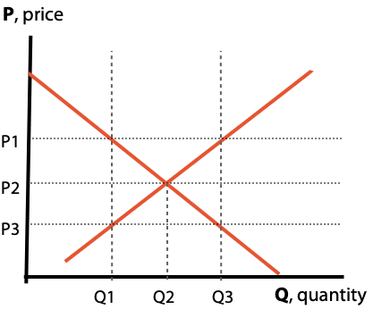
At a price of P1, Q3 will be made, but only Q1 demanded. There is excess supply and this will drive down the selling price, increasing demand. Prices will stabilise at a price of P2 and demand of Q2 where supply and demand match.

At a price of P3, Q3 is demanded but only Q1 supplied. There is excess demand and this will push up the price of goods until, again, demand and supply match at the price of P2.

5 Shifting the demand and supply curves

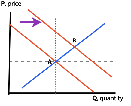
The diagram below shows a rightward shift in the demand curve.

5.1 A rightward shift in a demand curve can be caused by:

• Rise in income (more income implies more demand at a given price)

• Rise in the price of substitutes (will increase the attractiveness of this product)

• Rise in the expected price of the product (stocking-up now)

• Reduction in the price of complements (as more complements are bought so more of the product is bought)

• Change in tastes (an item can become fashionable or otherwise popular)

• Population increase (more people pursuing the goods).

As the demand curve shifts to the right more goods are demanded at the same price or the same quantity would demanded at a higher price. Once again supply will adjust so that a new equilibrium point is reached where demand and supply match. The equilibrium point moves from A to B above in the above diagram.

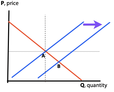
The diagram below shows a rightward shift in the supply curve, meaning that more goods will be produced at the same price or the same number of goods will be produced at a lower price.

5.2 A rightward shift in a supply curve can be caused by:

• Fall in cost of production

• Fall in the price of other goods

• Technology changes

• Improved efficiency

• Subsidies

• Lower taxes

If more goods are produced then to sell them the price will have to fall until equilibrium is reached again. The equilibrium point moves from A to B in the diagram above.

6 Cost curves

There are two types of cost:

Fixed costs:   do not vary in the short run as production increases.

For example, factory rent.

Variable costs:   increase with production volume.

For example, labour costs.

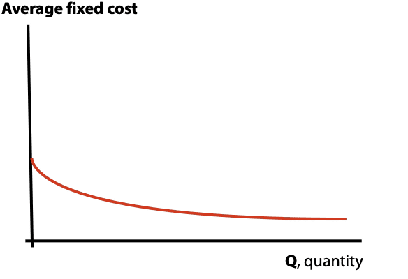
As production costs increase, the average fixed cost (the fixed cost per unit) will decrease because the constant fixed costs are being spread over more units. A graph of fixed cost per unit against output would look like:

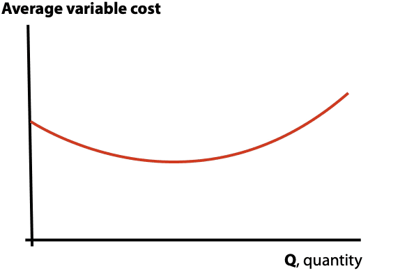
Initially variable costs per unit will fall as the producer gains advantages from greater efficiencies as more units are produced. Eventually the variable cost per unit increases because of the law of diminishing returns. For example, as machines are run harder more repairs are needed and the machine efficiency decreases. This is the law of diminishing returns.

A graph of variable cost per unit will look like:

Combining the graphs will produce:

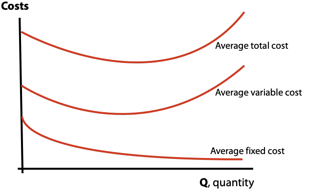
Provided the selling price is above the average variable cost the firm will produce even if the price is below the average total cost. For example, it would be worth producing and item for an additional cost of $7 if it sold for $10. The $3 difference helps towards covering fixed costs.

The marginal cost is the cost of producing an extra unit.

If average total costs are falling, the marginal cost must be less than the prevailing average so that the average cost is pulled down. If average total costs are rising, marginal costs must be greater than the prevailing average to increase the average. The marginal cost line will therefore go through the minimum point of the average total cost line. Similarly for average variable costs.

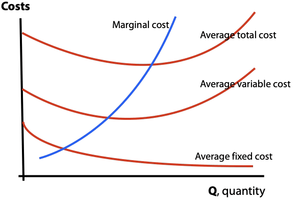
In the long run, all costs are variable and fixed capacity can be increased so that the law of diminishing returns will no longer apply. Indeed, increased capacity could bring economies of scale so that the supply curve could even be downward sloping.

7 Types of competition

7.1 Perfect competition

Many small buyers and sellers, none of which is large enough to affect the market or the market price.

Free entry and exit from the market.

Buyers and sellers are ‘price-takers’: the market price rules ie the equilibrium price. If a supplier raises its price, no-one will buy form that source as there a plenty of other suppliers. There is no point in lowering selling price because the seller sells all that can be made at the market price.Every buyer can buy what they want at the market price.

7.2 Imperfect competition

• Monopolist: only one supplier. The price can be set at any level to maximise revenue or profits, but volume demanded will change. Profits are, of course, not guaranteed as the monopolist might be selling something no-one wants.

• Oligopoly: a small number of suppliers (eg petrol companies). If a supplier raises prices, the others will win market share by sticking at the old price. If a buyer lowers the price the other have to follow to maintain market share.

• Monopolistic competition (non-price competition): where firms seek to increase demand for their products using something other than price. For example, brand and reputation can be used. An example is found in the car industries. Ford, General Motors, Nissan and VW all sell ‘family sized’ cars so are competing with each other. However, their prices differ so they are using factors other than price to generate sales. For example, VW will emphasise the engineering quality of its cars.