
Linear Programming

1 Introduction
Chapter 5 dealt with a shortage of ONE resource, and the answer there was a ranking: contribution, or throughput, per unit of the scarce resource. That method depends on being able to work down a list, giving each product all it can sell before moving to the next, and it stops working the moment a second resource is also short — because the product that is best per machine hour need not be the product that is best per kilogram, and a plan cannot follow both rankings at once.
Where two or more resources are limiting, the technique is linear programming. It is called linear because every relationship in it is a straight line: contribution per unit does not change with volume, and each unit of a product consumes the same quantity of each resource however many are made.
There are two ways of solving a linear programming problem. The simplex method works entirely with numbers and copes with any number of products; it is not in the P1 syllabus. The graphical method handles two products and is the one to know. It is unlikely that a whole problem would be set in one objective test question, but any step in it can be, and the steps only make sense once the whole thing has been seen through from beginning to end — which is what this chapter does with a single example.
Syllabus
This chapter completes P1C3c — product mix decisions with constraints for the case of two or more constraints. Chapter 5 carries the single-constraint case, and the shadow price in section 5 is the general form of the "most worth paying for one more unit" calculation that chapter 5 does in one line.
2 Formulating the problem
Formulation is writing the problem down in algebra, and it is worth doing carefully because everything afterwards depends on it. It is also the step most likely to be examined on its own.
The six steps
Define the variables — say what each letter stands for, and in what period.
Formulate an equation for the objective function — what is being maximised or minimised.
Formulate an inequality for each constraint, including the non-negativity constraints.
Graph the constraints, shade the feasible region and label its vertices.
Plot an iso-contribution line and slide it out to find the optimum vertex.
Confirm the exact solution by solving the two constraints that meet at that vertex as simultaneous equations.
2.1 Define the variables
Give each product a letter and say exactly what it counts, including the period. Any letters will do — x and y are as good as anything — but letters that mean something are easier to keep straight in a hurry. A separate letter is usually given to the objective as well.
2.2 The objective function
An equation for the thing to be maximised or minimised, in terms of the variables. In a short-term product-mix problem it is almost always contribution, for the reason given in chapter 5: the total fixed cost does not change with the plan, so maximising contribution maximises profit. The objective function is an equation, not an inequality, and it has no limit in it — its value is what is being sought.
2.3 The constraints
One inequality for each limitation. For a resource, add up what the plan would use and set it against what is available:
the quantity each product uses of the resource, multiplied by the number of that product, added across the products;
then “less than or equal to” the quantity available — not “equal to”, because there is no obligation to use it all;
demand limits are constraints in the same form (E ≤ 10), and demand that is unlimited simply produces no constraint;
a minimum requirement — a contract to supply at least so many units — is a “greater than or equal to” constraint.
Finally, the non-negativity constraints: every variable must be greater than or equal to zero. They look trivial and they are not optional. The algebra does not know that a negative number of chairs is impossible, and a question that asks for the constraints to be listed expects them.
This lecture is the formulation step, worked on Example 1. One correction before you watch: at the start the tutor refers back to the single-limiting-factor chapter as “chapter three, I think”. In the current notes that is chapter 5 — the recording was made under an earlier chapter numbering in which limiting factor analysis was chapter 3. Everything else in the recording is sound, and the constraints it derives are the ones in Answer 1 below.

Formulate and solve
Peter makes two types of chair — the ‘Executive’ and the ‘Standard’.
The data relating to each is as follows:
Per chair | Standard | Executive |
Materials | 2 kg | 4 kg |
Labour | 5 hours | 6 hours |
Contribution | $6 | $9 |
There is a maximum of 80 kg of material available each week and 180 labour hours per week. Demand for ‘Standard’ chairs is unlimited, but maximum weekly demand for ‘Executive’ chairs is 10.
Find the optimal production plan, which will maximise contribution, and state the contribution value that will be generated.
Show answerHide answer
3 The graphical solution
The graph does not produce the answer by itself — the exact values come from simultaneous equations — but it is what identifies which two lines to solve, and it is the step most likely to be tested by giving you a completed graph and asking you to read it.
3.1 Drawing a constraint
Put one variable on each axis. Every point in the space then represents a possible production plan, and each constraint divides that space in two.
Draw the line at which the constraint is exactly met. Because there is no squared or cubed term, that line is straight, and two points fix a straight line. The easiest two are the ends: set one variable to zero and solve for the other, then the other way round. Join them.
Then decide which side of the line satisfies the constraint. For a "less than or equal to" resource constraint it is the side towards the origin: on the line the resource is exactly used up, and below it less is used.
3.2 The feasible region
The feasible region is the area that satisfies every constraint at once. Any plan inside it or on its edge is possible; anywhere outside it at least one constraint is broken. It is normal for it to be bounded by only some of the lines drawn — a constraint that lies entirely outside the region formed by the others is redundant and can never bind.
Label the vertices — the corners — as you go. They are what the rest of the method works with.
3.3 The objective, or iso-contribution, line
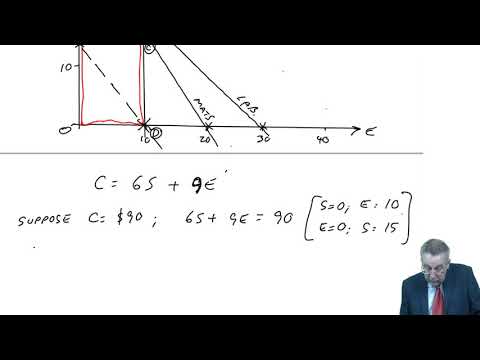
The value of C is not known yet, so pick any convenient value, draw the line for it, and use its slope. Choosing C = 90 in Example 1 gives 6S + 9E = 90, which passes through (0, 10) and (15, 0). Choosing C = 120 gives a line through (0, 13.33) and (20, 0) — a different line, and parallel to the first, because the slope is set by the 6 and the 9 and not by the value of C.
That is the whole trick. Every contribution line is parallel to every other, and the larger the contribution the further the line lies from the origin. It is called the iso-contribution line because every point along it gives the same contribution — “iso” meaning same.
3.4 Finding the optimum
Slide the contribution line outwards, keeping it parallel, until it is about to leave the feasible region. The last point it touches is the optimum. Because the region is a polygon, that point is always a vertex — and which vertex it is depends on the slope of the contribution line, so a flatter or steeper objective can move the answer to a different corner of the same region.
Then get the exact figures algebraically. Reading them off the graph is not accurate enough: in Example 1 the graph suggests roughly 25 or 26 standard chairs and the true answer is 30. Identify the two lines that cross at the optimum vertex and solve them as simultaneous equations.
Solving every pair of lines and taking the best result is not a substitute for drawing the graph. Two lines can cross at a point that is not in the feasible region at all — in Example 1 the labour and demand lines meet at a point that breaks the materials constraint — and a candidate list built without the graph will contain such points and may pick one of them.
This is the graphical solution of Example 1, worked on screen. Two things to know. The recording is titled “Shadow prices”, but shadow prices are in part 3 — this part covers the graph, the feasible region, the iso-contribution line and the simultaneous equations, i.e. sections 3.1 to 3.4. And the tutor reads roughly “five Es and 25, 26 Ss” off a hand-drawn graph before solving it properly; he says at the time that his graph is not accurate, and the correct answer, which he reaches a minute later, is 30 standard chairs and 5 executive.
4 Spare capacity: slack
A resource shortage does not oblige the optimum plan to use every unit of every resource. Where the plan uses less than the amount available, the difference is slack.
A constraint that is exactly met at the optimum is binding, and its slack is nil.
A constraint that is not exactly met has slack equal to the amount available less the amount used.
Slack is measured in the units of the constraint — kilograms, hours, or units of demand.
The quickest way to find it is to notice which lines the optimum vertex lies on: a vertex sitting on a constraint line uses that resource in full, so the slack is nil without any arithmetic. Only the constraints the vertex is not on need a calculation.
This lecture covers sections 4 and 5 — slack and shadow prices — worked on Examples 2 and 3, and its arithmetic agrees with the answers below throughout. One slip to know about: part-way through the shadow-price discussion the tutor says “it says here we’ve only got 18 kilos of material available”. It is 80 kg, as he says correctly both before and after.

Slack
Using the information from Example 1, calculate the slack for each of the constraints, i.e. for materials, for labour, and for demand for ‘Executive’ chairs.
Show answerHide answer
5 Shadow prices
In practice almost no resource is absolutely fixed. More material can usually be bought if a premium is paid for it, and more labour hours obtained by paying overtime. The question is how much extra is worth paying, and the answer is the shadow price.
Definition
The shadow price — also called the dual price — of a limited resource is the maximum PREMIUM worth paying, over and above the normal price, for one more unit of it. It equals the extra contribution earned if one more unit were available.
5.1 Calculating a shadow price
Add one unit to the constraint being examined, leave every other constraint alone, re-solve for the new optimum, and take the increase in contribution. In full:
increase the right-hand side of that one constraint by one unit;
solve it with the other constraint that meets it at the optimum vertex — the optimum stays at the intersection of the same two lines, because one extra unit moves the line only very slightly;
compute the contribution at the new solution;
the shadow price is the new contribution less the old.
The shadow price is a PREMIUM, not a price. It is the most that could be paid ON TOP OF the normal cost of the resource, because the contribution figures it is derived from already charge the resource at its normal price. If material normally costs $5 a kg and its shadow price is $1.125, the most worth paying for an extra kilogram is $6.125 — and at exactly that figure the business is no better off.
It follows that a resource with slack has a shadow price of nil. There is already more of it than the plan uses, so an extra unit changes nothing and is worth no premium at all. Only a binding constraint can have a shadow price.
5.2 How far a shadow price holds
A shadow price is not a rate that applies for ever. It holds only while the optimum stays at the intersection of the same two constraints. As more of the resource is added the optimum vertex slides along the other line, and at some point a third constraint becomes binding — beyond which the extra units are worth less, and the shadow price has to be recalculated. Answer 3 works out where that point is for both resources in the example.
Beyond P1. P1C3c asks for product mix decisions with constraints, and the examinable core of this chapter is formulating the problem, reading the graph and solving for the optimum. Shadow prices are taught here because the chapter’s own example asks for them and because they are the general form of the “most worth paying” calculation in chapter 5; the fuller treatment of linear programming duality, including sensitivity over the whole range of the right-hand sides, belongs to P2.
Shadow prices
Using the information from Example 1, calculate the shadow price of each of the constraints, i.e. for materials, for labour, and for demand for ‘Executive’ chairs.
Show answerHide answer
6 Non-integer answers
Linear programming regularly produces fractional answers: 5.625 executive chairs in Answer 3, and 29.25 standard chairs. That is not a mistake and it should not be rounded away.
The constraints in these problems are stated per week, so the solution is a rate per week, and a rate per week can perfectly well be an average. Producing 5.625 executive chairs a week means finishing five in one week and part of a sixth, and completing that one early in the next. Rounding down loses contribution and rounding up breaks a constraint, so unless the question specifically calls for whole units, leave the answer as it comes out.
7 Test your knowledge
Two quick checks before you move on: work through the flashcards to fix this chapter’s key terms and definitions, then sit the objective questions for exam-style practice. Both mark themselves and explain the answers as you go.
Linear Programming
12 questionsAnswer the questions one at a time. Your progress is saved so you can leave and come back.
Open chapter practice