Prices

1 Introduction to price behaviour

YouTube videoLoad YouTube video

Microeconomics is the branch of economics that deals with the price and the cost of individual goods, and with the way suppliers and customers react to prices.

It is close to self-evident that as the price of a product rises, the quantity demanded is likely to fall. If airfares rise, fewer people choose to travel. If a market trader is left at the end of the day with fruit that will not keep, the price comes down to stimulate demand.

This chapter looks at how price and quantity depend on one another on the demand side, at how price affects supply — higher prices encourage more production — and at how the price mechanism brings the two together so that demand equals supply.

2 Demand

2.1 The demand curve

For most goods, as the price increases the quantity demanded falls. Plotted with price on the vertical axis and quantity on the horizontal, that gives the DEMAND CURVE.

The curve is drawn as a straight line here for simplicity. In practice a demand curve is usually curved, because the responsiveness of demand to price is not the same at every price — section 3.3 shows exactly that.

There is one familiar exception to the downward slope. For a few luxury goods, a high price is part of what the buyer is paying for: the price signals exclusivity, and cutting it can reduce demand rather than increase it.

2.2 Movements along the curve and shifts of the curve

A shift to the right means more is demanded at every price; a shift to the left means less.

In the diagram, D is the original demand curve and the dashed D1 is the same demand after a rightward shift.

A shift can be caused by any of the following.

• CONSUMERS’ INCOME. In general, higher incomes shift the demand curve to the right, so that more is sold at any given price. There are exceptions, known as INFERIOR GOODS, whose demand curve shifts LEFT as income rises because buyers switch to something better. The demand for the cheapest brands of coffee falls as incomes rise and consumers move to premium brands.

• SUBSTITUTES AND COMPLEMENTS. A SUBSTITUTE is a product that can be bought instead: olive oil and sunflower oil are substitutes for many purposes, so if the price of olive oil rises, the demand for sunflower oil increases and its curve shifts right. COMPLEMENTS are bought together: cars and petrol. If the price of cars falls, more are bought and more petrol is bought too, even though the price of petrol has not changed, so petrol’s demand curve shifts right.

• FASHION AND TASTE. A fashionable item has high demand and consumers may be willing to pay a high price for it. Advertising works the same way: it increases the quantity demanded at any given price, shifting the curve to the right.

• EXPECTATIONS OF FUTURE PRICE CHANGES. If consumers think the price will rise, current demand increases as they buy ahead, and the curve shifts right. If they think it will fall, they wait, and it shifts left.

3 The price elasticity of demand

3.1 What elasticity means

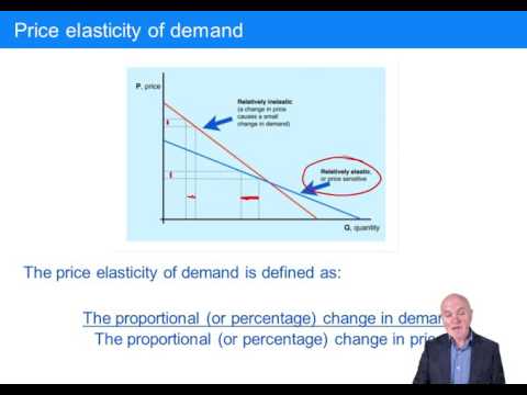
Elasticity determines the slope of the demand curve — how much the quantity demanded responds to a change in price.

If demand is ELASTIC, the good is price sensitive: a small change in price causes a relatively large change in demand. That is the flatter line below. If demand is INELASTIC, the good is price insensitive: a change in price has a relatively small effect on demand. That is the steeper line.

The measure itself is a ratio of two proportional changes:

3.2 Arc elasticity

There are two ways of calculating the elasticity between two points, and they differ only in what they measure the change AGAINST.

ARC ELASTICITY uses the MID-POINT of the two prices and of the two quantities as its base. Suppose that at a price of $8 demand is 1,200 units and at a price of $6 demand is 2,200 units.

Mid-point quantity = (2,200 + 1,200) ÷ 2 = 1,700. Mid-point price = ($8 + $6) ÷ 2 = $7.

Proportional change in demand = (2,200 − 1,200) ÷ 1,700 = 0.588, or 58.8%.

Proportional change in price = ($8 − $6) ÷ $7 = 0.286, or 28.6%.

Price elasticity of demand = 58.8 ÷ 28.6 = 2.06.

3.3 Point elasticity

POINT ELASTICITY uses the STARTING point as its base instead. On the same data, starting at a price of $8 and a demand of 1,200:

Proportional change in demand = (2,200 − 1,200) ÷ 1,200 = 0.833, or 83.3%.

Proportional change in price = ($8 − $6) ÷ $8 = 0.25, or 25%.

Price elasticity of demand = 83.3 ÷ 25 = 3.33.

The two methods give different answers on the same data — 2.06 and 3.33 — and neither is wrong. They are measuring the responsiveness against different bases. Read the requirement: if it says arc, use the mid-points; if it says point, use the starting values.

3.4 The determinants of the price elasticity of demand

The syllabus asks you to explain what MAKES demand elastic or inelastic. Six influences matter, and each of them is about how easy it is for the buyer to react to the price.

The influences interact, and the exam expects you to read a scenario for the one that dominates. Petrol has few substitutes and is hard to postpone, so its demand is inelastic in the short run — but it absorbs a large enough share of some household budgets, and has enough long-run substitutes, that its elasticity rises with time.

3.5 Price elasticity of demand and total revenue

The syllabus asks you to CALCULATE the effect of the price elasticity of demand on a firm’s total revenue, so the direction of the effect has to be worked out on figures rather than remembered as a rule.

Take a demand schedule in which quantity increases by 1,000 units for each $1 the price is cut, and add a column for total revenue, which is simply price × quantity.

Revenue rises as the price is cut from $12, peaks at $72,000 between $9 and $8, and then falls away. The total revenue curve is the inverted U below, drawn against quantity.

Now compute the arc elasticity at three places on the same schedule, and the shape of that curve stops being a coincidence.

Two cautions before you use this in an exam answer. Revenue is not profit: a price cut that raises revenue also raises the volume produced, and therefore the variable cost. And the schedule above assumes nothing else changes — if a competitor matches the price cut, the firm is no longer moving along its own demand curve, because the curve itself has shifted.

4 Supply

4.1 The supply curve, movements and shifts

As you would expect, the higher the price offered to suppliers, the more will be produced. Existing suppliers increase output and new suppliers enter the market, because at a higher price there is more profit in it. At a very low price only the single most efficient producer can survive; as the price rises, less efficient producers become viable too.

The same MOVEMENT-versus-SHIFT distinction applies as on the demand side. A change in the price of the good is a movement ALONG the supply curve. A change in anything else shifts the whole curve.

A shift to the right means that more is supplied at every price — or, read the other way, that the same quantity will now be produced for a lower selling price.

In the diagram, S is the original supply curve and the dashed S1 is supply after a rightward shift.

A rightward shift can be caused by:

• LOWER AVERAGE COSTS OF PRODUCTION, so that producing the same volume is still worthwhile even if selling prices fall;

• SUBSIDIES for raw materials or labour, or lower tax and duty on purchases, which have the same effect on cost;

• MORE EFFICIENT USE OF THE EXISTING FACTORS OF PRODUCTION — ordering materials more accurately, rearranging work rotas — which again lowers the cost of production; and

• IMPROVEMENTS IN TECHNOLOGY, such as more efficient processes or automation.

A shift to the LEFT, in which less is supplied at every price, can be caused by:

• an increase in the average cost of production;

• taxation of raw materials;

• a government quota or other restriction on how much may be produced; or

• a switch of production to more profitable products, which simply removes productive capacity from this market.

4.2 The price elasticity of supply and its determinants

It is calculated exactly as the price elasticity of demand is, and the same choice between the arc and the point method applies. Because a higher price normally brings out more supply, the result is positive.

Supply is likely to be ELASTIC if:

• there is spare capacity in producers’ factories;

• there is inventory available that can easily be released and sold;

• it is easy to employ more factors of production; and

• additional sources of the product are easy to create.

Supply is likely to be INELASTIC if:

• suppliers are already operating close to full capacity;

• stocks are low, so there are no surplus goods to sell;

• additional sources of supply are difficult to create — expensive, complex factories are needed;

• it is difficult to employ the factors of production, for example because highly skilled labour is needed and is scarce; and

• the product takes time to produce. Agricultural supply is inelastic in the short run because food takes a season to grow; only imports can relieve a shortage before the next harvest.

As with demand, TIME is the influence that runs through all of these: supply is nearly always more elastic in the long run than in the short run, because given long enough a producer can build the factory, train the workers or plant the crop.

5 The equilibrium price

Putting the demand and supply curves on the same axes gives the price mechanism itself.

D is the demand curve and S the supply curve.

At the price where the two curves cross, the quantity suppliers wish to supply is exactly the quantity buyers wish to buy. That price is the EQUILIBRIUM PRICE and that quantity is the equilibrium quantity. At any other price the market is in DISEQUILIBRIUM, and the price mechanism moves it back.

5.1 Excess demand

Suppose the market price is P1, below the equilibrium.

At P1 the quantity demanded, read off the demand curve, is larger than the quantity supplied, read off the supply curve. The difference between them is the EXCESS DEMAND.

The market is now in disequilibrium, and it corrects itself. Some buyers who cannot obtain the good offer more for it, so the price RISES. The higher price both encourages suppliers to produce more and discourages some buyers, and the two movements continue until the excess demand has gone and equilibrium is restored.

5.2 Excess supply

Now suppose the market price is P2, above the equilibrium.

At P2 the quantity supplied exceeds the quantity demanded, and the difference is the EXCESS SUPPLY.

Again the market corrects itself. Producers holding unsold goods lower their prices to clear them, so the price FALLS. The lower price increases the quantity demanded and makes production unattractive to the least efficient suppliers, who leave, until equilibrium is restored.

5.3 The same model in other markets

The syllabus asks for the equilibrium price in PRODUCT OR FACTOR markets, and the whole point of the model is that it is the same model in both. Everything in this chapter applies wherever a price is set by demand and supply:

The last row is worth dwelling on, because it is the whole chapter in one line: hotel rooms cannot be added for one weekend, so supply is almost perfectly inelastic in the short run, and any increase in demand is therefore absorbed almost entirely by the price.

6 Tests

The chapter’s own five questions follow. Work each one before you open the answer.

7 Test your knowledge

Two quick checks before you move on: work through the flashcards to fix this chapter’s key terms and definitions, then sit the objective questions for exam-style practice. Both mark themselves and explain the answers as you go.