
Pricing


1 Introduction
An important decision for the management accountant is that of fixing a selling price.
In this chapter we will consider the practical considerations that are likely to apply, and also some theoretical calculations that you need to know.
2 Factors influencing selling price
Many factors are relevant when considering what price to charge.
2.1 The main areas to be considered are the following:
costs
competitors
customers
3 Cost plus pricing
Using cost-plus pricing, the selling price is calculated by estimating the cost per unit of a product and adding an appropriate percentage mark-up.
A primary consideration will be as to what is to be regarded as the cost – full cost, marginal cost, or opportunity cost.
3.1 Full cost plus
Full cost includes a share of overheads and also often includes non-production costs.
advantages
disadvantages
3.2 Marginal cost plus
The price of the product is determined by calculating the marginal (or incremental) cost of producing a unit and adding a mark-up.
advantages
disadvantages
3.3 Opportunity cost plus
This is a marginal cost approach but also includes within the cost any opportunities foregone. It is a relevant costing approach.
A new product is being launched, and the following costs have been estimated:
Materials $10 per unit
Labour $8 per unit
Variable overheads $5 per unit
Fixed overheads have been estimated to be $50,000 per year, and the budgeted production is 10,000 units per year.
Calculate the selling price based on:
full cost plus 20%
marginal cost plus 40%
4 Optimal pricing – tabular approach

One major disadvantage of a cost plus approach to pricing is that it completely ignores the possible effect of the selling price on the level of demand.
For many products (but not all) it is the case that a higher selling price will result in lower demand, and vice versa.
It could therefore be worthwhile to reduce the selling price and sell more – provided of course that this resulted in a higher total profit.
Kennedy plc has established that the price demand relationship is as follows:
S.P. p.u. | Demand |
16 | 100 |
15.5 | 200 |
15 | 300 |
14.5 | 400 |
14 | 500 |
13.5 | 600 |
13 | 700 |
They have also established that the cost per unit for production of jars of coffee is as follows:
Quantity | Cost p.u. |
100 | 14.0 |
200 | 13.9 |
300 | 13.8 |
400 | 13.7 |
500 | 13.6 |
600 | 13.5 |
700 | 13.4 |
800 | 13.3 |
900 | 13.2 |
Determine the optimal selling price in order to maximise profit
S.P. p.u. | Demand | Cost p.u. | Total Revenue | Total Cost | Total Profit | Marginal Revenue | Marginal Cost |
Whichever way you choose to calculate the optimum selling price in the above example, do be aware that it occurs at the point where marginal revenue = marginal cost. You could be specifically asked to use this fact in the examination.
5 Price elasticity of demand
In the previous example, a reduction in the selling price results in an increase in demand (and vice versa). This is true of many products, but the effect of selling price on demand will be different for different products. The effect of selling price on demand is also likely to be different for the same product at different levels of selling price.
A measure of the size of the effect on demand of a change in selling price is called the price elasticity of demand.
A high PED means that the demand is very sensitive to changes in price, or elastic.
A low PED means that the demand is not very sensitive to changes in price, or inelastic.
Using the figures from example 2, calculate the price elasticity of demand
if the current selling price is $16 per unit
if the current selling price is $15 per unit
6 Optimal pricing – equations

In section 4, we were presented with the price/demand relationship as a table, and used these figures to calculate the optimum level of selling price from those available.
In principle, it would be possible to have an equation relating the selling price to the demand, and to then solve the problem algebraically.
6.1 Price/demand equation
In the exam you could be asked to derive the price/demand equation yourself from information given, or alternatively you could be given the equation. If you were asked to derive the equation yourself, then it would always be on the basis that the relationship was linear (as is the case in example 2, from inspection).
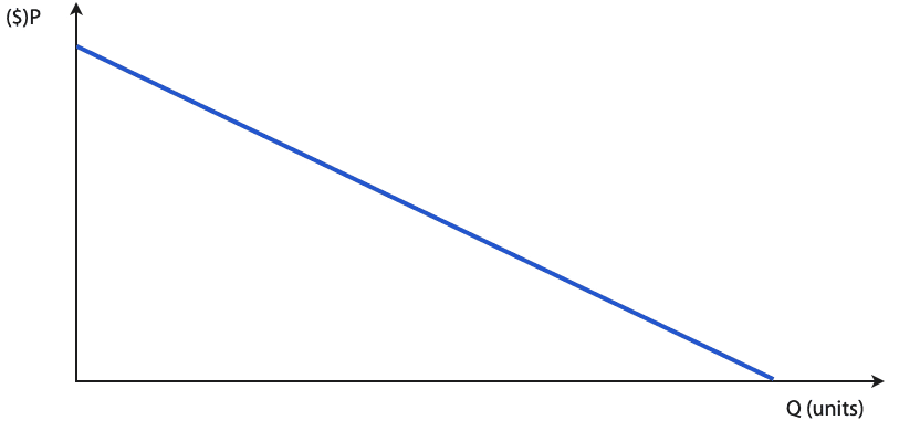
The equation would therefore be of the form:
P = a – bQ
where:
P = selling price
Q = quantity demanded at that price
a = theoretical maximum price (if the price is set at ‘a’ or above, then the demand will be zero)
b = the change in price required to change demand by 1 unit (the gradient of the line)
A company sells an article at $12 per unit and has a demand of 16,000 units at this price.
If the selling price were to be increased by $1 per unit, it is estimated that demand will fall by 2,500 units.
On the assumption that the price/demand relationship is linear, derive the equation relating the selling price to the demand.
6.2 Optimal selling price
Having identified the price/demand relationship, it is easy to derive the equation for the revenue at any level – the total revenue will be equal to PQ.
We could then show on a graph the total revenue and total costs for any level of demand. It would be of this sort of shape:
Our objective is to maximise profit. We can do this by calculating the Marginal Revenue and Marginal Cost, and using the fact that the profit is maximised when the two are equal.
A company currently has a demand for one of its products of 2000 units at a selling price of $30 per unit.
It has been determined that a reduction in selling price of $1 will result in additional sales of 100 units.
The costs of production are $1000 (fixed) together with a variable cost of $20 per unit.
(Note: see the note at the top of the next page)
Calculate the selling price p.u. at which the profit will be maximised.
Note: you cannot be required to differentiate in the examination, and therefore the formula for the marginal revenue is given on the formula sheet: MR = a – 2bQ
At a selling price of $100 p.u. the company will sell 20,000 units p.a..
For every $2 change in the selling price, the demand will change by 2,000 units.
The costs comprise a fixed cost of $100,000, together with a variable cost of $5 p.u..
Calculate the selling price p.u. that will result in maximum profit p.a., and the amount of that profit.
7 Pricing strategies

In particular circumstances, for particular reasons, the company may decide on a special strategy with regard to its pricing policy.
You should be aware of the following common strategies, and be able to give examples of circumstances where they may be considered.
Penetration pricing
Price skimming
Product-line pricing
Complementary products
Price discrimination
Volume discounting
Where a requirement names pricing strategies, take each in turn: explain it, apply it to the scenario’s own facts — a patent-protected product for skimming, spare parts and servicing for complementary pricing, countries with different elasticities for discrimination — and conclude whether the company could use it. A strategy nobody asked about earns nothing.
Pricing
10 questionsAnswer the questions one at a time. Your progress is saved so you can leave and come back.
Open chapter practice