
The Normal distribution

1 Introduction
We discussed probabilities in a previous chapter. In this chapter we will see how tables may be used to calculate probabilities for certain frequency distributions.
2 The histogram revisited
You should remember from the last chapter what the histogram is, and how it is drawn. Importantly, it is the area of the bars that is proportional to the frequency.
The following table shows the annual salaries earned by 150 workers.
Salary | Frequency |
$0 - $1,000 | 25 |
$1,000 - $2,000 | 35 |
$2,000 - $3,000 | 40 |
$3,000 - $5,000 | 50 |
150 |
Show this frequency table in the form of a histogram
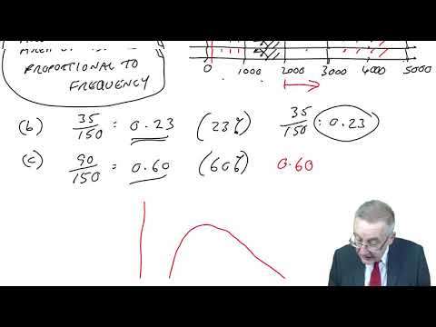
Calculate the probability of a worker earning between $1,000 and $2,000
Calculate the probability of a worker earning more than $2,000
Show answerHide answer
We can easily calculate the probabilities from the frequency table. However, if we were presented an accurately drawn histogram, then even without the original table we could still calculate the probability of a worked earning within a specific range.
The area of all the bars is proportional to the total number of workers, and the area of the bars representing any specific range is proportional to the number of workers earning within that range. We could calculate the probability by dividing the area of the bar(s) representing the specific range by the total area of all the bars.
3 The normal distribution
The normal distribution is effectively a ‘smoothed-out’ histogram with a very specific shape.
The main features of a normal distribution are:
it is symmetrical about the mean
it is continuous
the mean coincides with the mode
it is ‘bell-shaped’
For a distribution that is shaped normally, we can calculate the areas under the curve as a proportion of the total area (and therefore the probabilities) by using normal distribution tables (which you will be provided with in the exam).
The normal distribution tables give us the area under the curve between the mean and some other point above or below the mean.
The size of the areas we are at for will depend on how great or small the spread of the distribution is, and therefore when we use the tables we look at the number of standard deviations we are from the arithmetic mean.
We call this distance the z-score.
A company produces units with an average length of 10 cm, and a standard deviation of
0.2 cm
What proportion of the units will have a length of:
more that 10 cms
between 10 and 10.4 cms
less than 9.8 cms
Show answerHide answer
It is also possible to use the normal distribution tables ‘backwards’.
For the same information as in Example 2, there is a 0.95 (or 95%) probability that the length will be more than X cms.
Calculate a value for X (remember that there is a 0.5 (or 50%) probability of the length being more than the average of 10 cms, because the normal distribution is symmetrical).
Show answerHide answer
The Normal Distribution
5 questionsAnswer the questions one at a time. Your progress is saved so you can leave and come back.
Open chapter practice